Upscaling unstructured grids
This notebook presents how to upscale a fine structured grid to a coarse unstructured grid using uppy. Grid are generated using flopy and gridgen.
Note that grid cells need to be rectangles.
Multiple type of grids are presented:
2D DISV grid (see modflow 6 documentation)
3D DISV grid
3D DISU grid
[1]:
import os
import sys
import numpy as np
import matplotlib.pyplot as plt
import flopy
from flopy.utils.gridgen import Gridgen
from flopy.export.vtk import Vtk
# import pyvista as pv

%load_ext autoreload
%autoreload 2

# import uppy
sys.path.append("../../")
import ArchPy
import ArchPy.uppy
from ArchPy.uppy import upscale_k, upscale_k_2D, rotate_point
[2]:
from ArchPy.C_modules.simplified_renorm_C import simplified_renorm3D
[3]:
gridgen_path = "../../../../exe/gridgen.exe"
2D DISV
Let’s create a 2D unstructured grid using gridgen and flopy
[4]:
# grid dimensions
nlay = 1
nrow = 8
ncol = 8
delr = 100.
delc = 100.
top = 0.
botm = -100.


sim = flopy.mf6.MFSimulation(
    sim_name="asdf", sim_ws="ws", exe_name="mf6")
tdis = flopy.mf6.ModflowTdis(sim, time_units="DAYS", perioddata=[[1.0, 1, 1.0]])
ms = flopy.mf6.ModflowGwf(sim, modelname="asdf", save_flows=True)
dis = flopy.mf6.ModflowGwfdis(
    ms,
    nlay=nlay,
    nrow=nrow,
    ncol=ncol,
    delr=delr,
    delc=delc,
    top=top,
    botm=botm,
    xorigin=1103.3,
    yorigin=1103.5,
)

# create Gridgen object
g = Gridgen(ms.modelgrid, model_ws="gridgen_ws", exe_name=gridgen_path)  # ! modidfy path to gridgen.exe !

# polygon refinement in the center of the grid (size 250 x 250)
polygon = [
    [
        (1600, 1350),
        (1700, 1300),
        (1300, 1800),
        (1300, 1700),
        (1600, 1350),
    ]
]


g.add_refinement_features([polygon], "polygon", 3, range(nlay))  # refinement level
refshp0 = "gridgen_ws/" + "rf0"
[5]:
ms.modelgrid
[5]:
xll:1103.3; yll:1103.5; rotation:0.0; units:undefined; lenuni:0
Build refinement
[6]:
g.build(verbose=False)
grid = flopy.discretization.VertexGrid(**g.get_gridprops_vertexgrid())
[7]:
grid.ncpl # number of cells
[7]:
523
[8]:
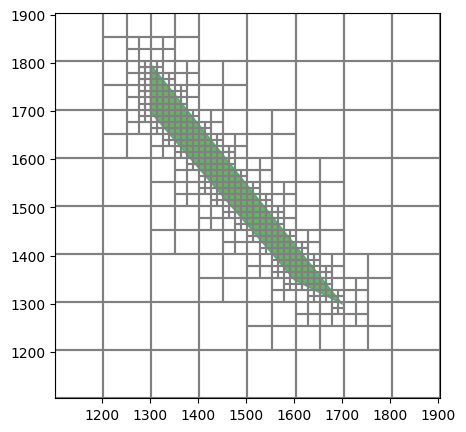
fig = plt.figure(figsize=(5, 5))
ax = fig.add_subplot(1, 1, 1, aspect="equal")
mm = flopy.plot.PlotMapView(model=ms)
grid.plot(ax=ax)

flopy.plot.plot_shapefile(refshp0, ax=ax, facecolor="green", alpha=0.6)
Possible issue encountered when converting Shape #0 to GeoJSON: Shapefile format requires that polygons contain at least one exterior ring, but the Shape was entirely made up of interior holes (defined by counter-clockwise orientation in the shapefile format). The rings were still included but were encoded as GeoJSON exterior rings instead of holes.
[8]:
<matplotlib.collections.PatchCollection at 0x22cea37d250>
[9]:
disv_gridprops = g.get_gridprops_disv() # get the disv gridprops
[10]:
# remove existing dis package and add new disv package
ms.dis.remove()
disv = flopy.mf6.ModflowGwfdisv(ms, **disv_gridprops, xorigin=0, yorigin=0)  # it is important to set xorigin and yorigin to 0, 0
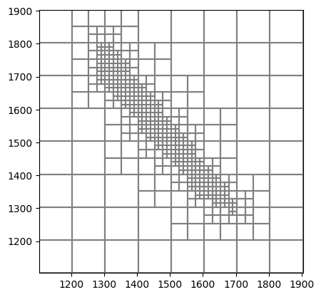
[11]:
ms.modelgrid.plot()
[11]:
<matplotlib.collections.LineCollection at 0x22ced7e8bd0>
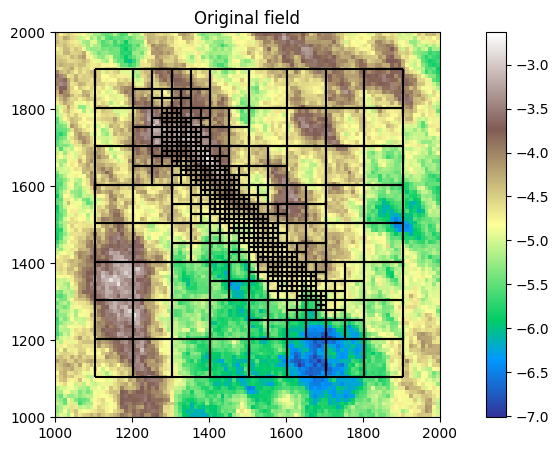
Now we generate a reference K field. Note that the field that is upscaled must be larger (or equivalent), in extension, than the new coarse grid
[12]:
# generate a random field for the grid
import geone

np.random.seed(16)

cm = geone.covModel.CovModel2D(elem=[("spherical", {"w":.5, "r":[250, 450]})
                                    ], alpha=30,
                                name="model")
nx_grid, ny_grid = 100, 100
sx_grid, sy_grid = 10, 10
ox_grid, oy_grid = 1000, 1000
field = geone.multiGaussian.multiGaussianRun(cm, (nx_grid, ny_grid), (sx_grid, sy_grid), (ox_grid, oy_grid), output_mode="array", mean=-5)
grf2D: Preliminary computation...
grf2D: Computing circulant embedding...
grf2D: embedding dimension: 128 x 256
grf2D: Computing FFT of circulant matrix...
[13]:
fig, ax = plt.subplots(1, 1, figsize=(12, 5))

grid.plot(ax=ax, color="k")

plt.imshow(field[0], cmap="terrain", vmin=field[0].min(), vmax=field[0].max(), extent=[ox_grid, ox_grid+sx_grid*nx_grid, oy_grid, oy_grid+sy_grid*ny_grid])
plt.xlim(ox_grid, ox_grid+sx_grid*nx_grid)
plt.ylim(oy_grid, oy_grid+sy_grid*ny_grid)
plt.colorbar()
plt.title("Original field")
plt.show()
Upscaling
The available method for the upscaling are:
arithmetic mean
harmonic mean
geometric mean
Simplified renormalization
Note that upscaling function (upscale_k_2D and upscale_k) need to be compiled first by numba. Hence the first call to the function will be slow.
[14]:
field = 10**field
[15]:
new_k = upscale_k_2D(field[0], dx=sx_grid, dy=sy_grid, ox=ox_grid, oy=oy_grid, method="simplified_renormalization", grid=grid)
[16]:
%%time
# new_k_g = upscale_k_2D(field[0], dx=sx_grid, dy=sy_grid, ox=ox_grid, oy=oy_grid, method="geometric", grid=grid)
# new_k_h = upscale_k_2D(field[0], dx=sx_grid, dy=sy_grid, ox=ox_grid, oy=oy_grid, method="harmonic", grid=grid)
# new_k_m = upscale_k_2D(field[0], dx=sx_grid, dy=sy_grid, ox=ox_grid, oy=oy_grid, method="arithmetic", grid=grid)
new_k = upscale_k_2D(field[0], dx=sx_grid, dy=sy_grid, ox=ox_grid, oy=oy_grid, method="simplified_renormalization", grid=grid)
CPU times: total: 62.5 ms
Wall time: 74.8 ms
C version is generally faster than pure python (between 2x-10x faster)
[17]:
%%time
# new_k_g = upscale_k_2D(field[0], dx=sx_grid, dy=sy_grid, ox=ox_grid, oy=oy_grid, method="geometric", grid=grid)
# new_k_h = upscale_k_2D(field[0], dx=sx_grid, dy=sy_grid, ox=ox_grid, oy=oy_grid, method="harmonic", grid=grid)
# new_k_m = upscale_k_2D(field[0], dx=sx_grid, dy=sy_grid, ox=ox_grid, oy=oy_grid, method="arithmetic", grid=grid)
new_k = upscale_k_2D(field[0], dx=sx_grid, dy=sy_grid, ox=ox_grid, oy=oy_grid, method="simplified_renormalization_C", grid=grid)
CPU times: total: 31.2 ms
Wall time: 29.4 ms
[18]:
new_k = upscale_k_2D(field[0], dx=sx_grid, dy=sy_grid, ox=ox_grid, oy=oy_grid, method="simplified_renormalization_C", grid=grid)
[19]:
new_k = np.log10(new_k)
Let’s compare to a standard upscaling using a structured grid
[20]:
%%time
Kxx, Kyy = upscale_k_2D(field[0], dx=5, dy=5, factor_x=5, factor_y=5)
CPU times: total: 109 ms
Wall time: 110 ms
[21]:
Kxx, Kyy = upscale_k_2D(field[0], dx=5, dy=5, factor_x=5, factor_y=5)
[22]:
Kxx = np.log10(Kxx)
Kyy = np.log10(Kyy)
[23]:
field = np.log10(field)
[24]:
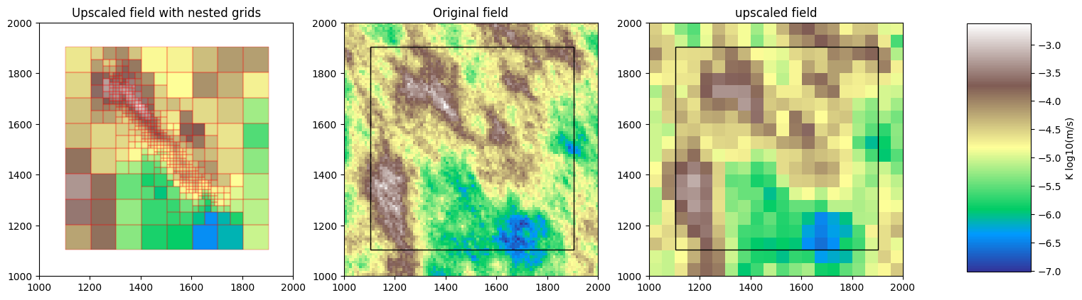
%matplotlib inline
fig, ax = plt.subplots(1, 3, figsize=(18, 5))

mm = flopy.plot.PlotMapView(model=ms, ax=ax[0])
mm.plot_grid(color="red", alpha=.15)
mm.plot_array(new_k[1], alpha=1, cmap="terrain", vmin=field[0].min(), vmax=field[0].max())
ax[0].set_xlim(ox_grid, ox_grid + 1000)
ax[0].set_ylim(oy_grid, oy_grid + 1000)
ax[0].set_title("Upscaled field with nested grids")
ax[0].set_aspect("equal")

ax[1].imshow(field[0], cmap="terrain", vmin=field[0].min(), vmax=field[0].max(), extent=(ox_grid, ox_grid + 1000, oy_grid, oy_grid + 1000))
#draw rectangle of the size of field
extent = ms.modelgrid.extent
x1, x2, y1, y2 = extent
rect = plt.Rectangle((x1, y1), x2 - x1, y2 - y1, edgecolor="black", facecolor="none")
ax[1].add_patch(rect)
# plt.colorbar()
# grid_ref.plot(alpha=.2, ax=ax[1])
ax[1].set_title("Original field")
ax[1].set_aspect("equal")

g = ax[2].imshow(Kyy, cmap="terrain", vmin=field[0].min(), vmax=field[0].max(), extent=(ox_grid, ox_grid + 1000, oy_grid, oy_grid + 1000))
# plt.colorbar()
rect = plt.Rectangle((x1, y1), x2 - x1, y2 - y1, edgecolor="black", facecolor="none")
ax[2].add_patch(rect)
ax[2].set_title("upscaled field")
ax[2].set_aspect("equal")

# add colorbar
fig.subplots_adjust(right=0.8)
cbar_ax = fig.add_axes([0.85, 0.15, 0.05, 0.7])
cl = fig.colorbar(g, cax=cbar_ax)
cl.set_label("K log10(m/s)")

plt.show()
3D DISV
Same as before but here using a 3D grid
[25]:
# 3D example
# grid dimensions
nlay = 4
nrow = 8
ncol = 8
delr = 100.
delc = 100.
top = 0.
ox = 1103.3
oy = 1103.5

botm = np.linspace(-10, -100, nlay)

sim = flopy.mf6.MFSimulation(
    sim_name="asdf", sim_ws="ws", exe_name="mf6")
tdis = flopy.mf6.ModflowTdis(sim, time_units="DAYS", perioddata=[[1.0, 1, 1.0]])
ms = flopy.mf6.ModflowGwf(sim, modelname="asdf", save_flows=True)
dis = flopy.mf6.ModflowGwfdis(
    ms,
    nlay=nlay,
    nrow=nrow,
    ncol=ncol,
    delr=delr,
    delc=delc,
    top=top,
    botm=botm,
    xorigin=ox,  # gridgen will be applied on a grid with origin at 0, 0
    yorigin=oy,
    angrot=0,
)

# create Gridgen object
g = Gridgen(ms.modelgrid, model_ws="gridgen_ws", exe_name=gridgen_path)

polygon = [
    [
        (1800, 1700),
        (1800, 1500),
        (1400, 1500),
        (1400, 1700),
        (1800, 1700),
    ]
]
polygon = np.array(polygon)

g.add_refinement_features([polygon], "polygon", 3, range(nlay))
refshp0 = "gridgen_ws/" + "rf0"
[26]:
g.build(verbose=False)
[27]:
ms.dis.remove()
disv_gridprops = g.get_gridprops_disv()
disv = flopy.mf6.ModflowGwfdisv(ms, **disv_gridprops, xorigin=0, yorigin=0)  # create grid this time with the origin at ox, oy
[28]:
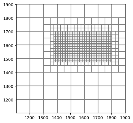
grid = ms.modelgrid
grid.plot()
[28]:
<matplotlib.collections.LineCollection at 0x22cee62b210>
[29]:
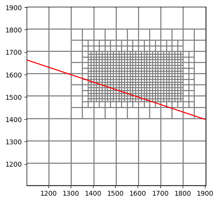
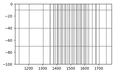
# plot a cross section
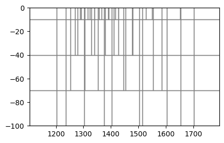
from flopy.plot import PlotCrossSection
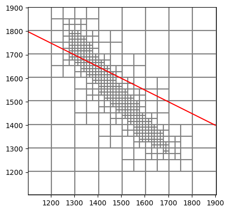
linex, liney = [700, 1900], [1800, 1400]
mm = flopy.plot.PlotMapView(model=ms)
ms.modelgrid.plot()
plt.plot(linex, liney, "r-")
plt.show()
fig = plt.figure(figsize=(4.8, 3))
xsect = PlotCrossSection(model=ms,geographic_coords=True, line={"line": [linex, liney]})
xsect.plot_grid()
[29]:
<matplotlib.collections.PatchCollection at 0x22cee4a1450>
[30]:
# generate a random field for the grid
import geone

np.random.seed(15)

cm = geone.covModel.CovModel3D(elem=[("spherical", {"w":1, "r":[250, 450, 50]})
                                    ], alpha=30,
                                name="model")

# grid parameters
nx_grid, ny_grid, nz_grid = 100, 100, 100
sx_grid, sy_grid, sz_grid = 10, 10, 1
ox_grid, oy_grid, oz_grid = 1000, 1000, -100
field_img = geone.multiGaussian.multiGaussianRun(cm, (nx_grid, ny_grid, nz_grid), (sx_grid, sy_grid, sz_grid), output_mode="img", mean=-5, algo="fft")
grf3D: Preliminary computation...
grf3D: Computing circulant embedding...
grf3D: embedding dimension: 128 x 256 x 128
grf3D: Computing FFT of circulant matrix...
[31]:
# pv.set_jupyter_backend('client')
[32]:
# create a modflow grid of the resolution of the random field to check the extent of the two grids

field = field_img.val[0]
field = np.flip(np.flipud(field), axis=1)  # flip the field to have the same orientation as the grid
nrow = field.shape[1]
ncol = field.shape[2]
nlay = field.shape[0]
botm = np.linspace(-1, -100, nlay)
# transform botm to have the same shape as the field
botm = np.repeat(botm.reshape(-1, 1, 1), nrow, axis=1)
botm = np.repeat(botm, ncol, axis=2)
top = np.zeros((nrow, ncol))
grid_ref = flopy.discretization.StructuredGrid(nrow=field.shape[1], ncol=field.shape[2], nlay=field.shape[0],
                                               delr=np.ones((field.shape[2]))*sx_grid, delc=np.ones((field.shape[1]))*sy_grid,
                                               botm=botm, top=top,
                                               xoff=1000, yoff=1000, angrot=0)
Check superposition of the two grids
[33]:
grid = ms.modelgrid
grid_ref.plot(alpha=.1, color="blue")
grid.plot()
[33]:
<matplotlib.collections.LineCollection at 0x22cf1316fd0>

[34]:
field = 10**field
[35]:
grid.ncpl * grid.nlay # number of cells
[35]:
3088
[36]:
%%time
Kxx1, Kyy, Kzz = upscale_k(field, dx=sx_grid, dy=sy_grid, dz=sz_grid, ox=ox_grid, oy=oy_grid, oz=oz_grid, method="simplified_renormalization", grid=grid)
CPU times: total: 1.72 s
Wall time: 1.71 s
[37]:
%%time
Kxx2, Kyy, Kzz = upscale_k(field, dx=sx_grid, dy=sy_grid, dz=sz_grid, ox=ox_grid, oy=oy_grid, oz=oz_grid, method="simplified_renormalization_C", grid=grid)
CPU times: total: 188 ms
Wall time: 214 ms
[38]:
%%time
Kxx, _, _ = upscale_k(field, dx=sx_grid, dy=sy_grid, dz=sz_grid, ox=ox_grid, oy=oy_grid, oz=oz_grid, method="arithmetic", grid=grid)
CPU times: total: 125 ms
Wall time: 136 ms
[39]:
Kxx, Kyy, Kzz = upscale_k(field, dx=sx_grid, dy=sy_grid, dz=sz_grid, ox=ox_grid, oy=oy_grid, oz=oz_grid, method="simplified_renormalization_C", grid=grid)
[40]:
Kxx = np.log10(Kxx)
Kyy = np.log10(Kyy)
Kzz = np.log10(Kzz)
[41]:
sx_grid
[41]:
10
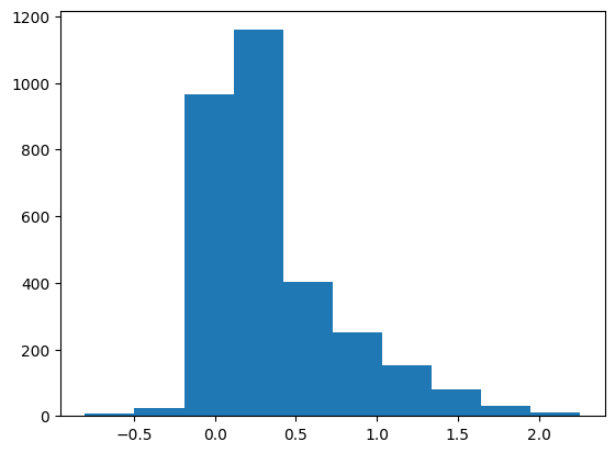
[42]:
plt.hist((Kxx - Kzz).flatten())
[42]:
(array([   8.,   23.,  967., 1159.,  404.,  251.,  152.,   81.,   31.,
          12.]),
 array([-0.80159967, -0.49586197, -0.19012428,  0.11561342,  0.42135112,
         0.72708882,  1.03282652,  1.33856422,  1.64430192,  1.95003962,
         2.25577732]),
 <BarContainer object of 10 artists>)
[43]:
%%time
field_kxx, fieldkyy, field_kzz = upscale_k(field, method="simplified_renormalization", dx=10, dy=10, dz=1, factor_x=5, factor_y=5, factor_z=5)
CPU times: total: 3.94 s
Wall time: 4.05 s
[44]:
%%time
field_kxx, fieldkyy, field_kzz = upscale_k(field, method="simplified_renormalization_C", dx=10, dy=10, dz=1, factor_x=5, factor_y=5, factor_z=5)
CPU times: total: 234 ms
Wall time: 232 ms
[45]:
field_kxx, fieldkyy, field_kzz = upscale_k(field, method="simplified_renormalization_C", dx=10, dy=10, dz=1, factor_x=5, factor_y=5, factor_z=5)
[46]:
field_kxx = np.log10(field_kxx)
field_kyy = np.log10(fieldkyy)
field_kzz = np.log10(field_kzz)
[47]:
# get number of cells in field_kxx
nlay = field_kxx.shape[0]
nrow = field_kxx.shape[1]
ncol = field_kxx.shape[2]
ncells = nlay*nrow*ncol
ncells
[47]:
8000
[48]:
vert_exag = 1
vtk = Vtk(model=ms, binary=False, vertical_exageration=vert_exag, smooth=True)
vtk.add_model(ms)
vtk.add_array(Kxx, name="K")
vtk.add_array(Kyy, name="Kyy")
vtk.add_array(Kzz, name="Kzz")
gwf_mesh = vtk.to_pyvista()
[49]:
ms.dis.yorigin = 0
ms.dis.xorigin = 0
[50]:
import pyvista as pv
pv.set_plot_theme("document")
pv.set_jupyter_backend('static')
pl = pv.Plotter(shape=(1, 3), window_size=[2000, 800])
pl.subplot(0, 0)
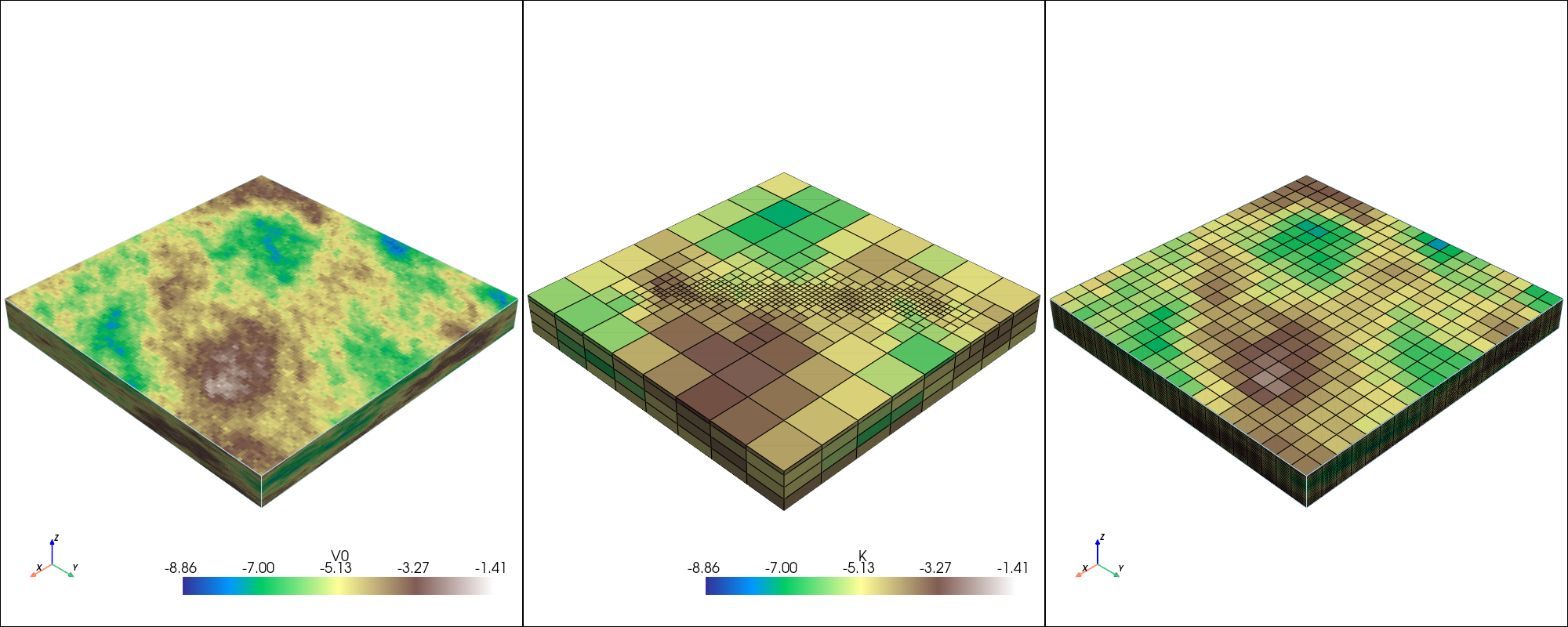
geone.imgplot3d.drawImage3D_surface(field_img, plotter=pl, cmap="terrain", opacity=1)
pl.subplot(0, 1)
pl.add_mesh(gwf_mesh, opacity=1, scalars="K", cmap="terrain", clim=[field_img.val.min(), field_img.val.max()], show_edges=False, show_scalar_bar=False)
pl.subplot(0, 2)
arr = field_kxx
arr = np.flipud(np.flip(arr, axis=1))
img = geone.img.Img(nx=arr.shape[2], ny=arr.shape[1], nz=arr.shape[0], sx=sx_grid*10, sy=sy_grid*10, sz=sz_grid*10, ox=0, oy=0, oz=-100, nv=1, val=arr.flatten())
geone.imgplot3d.drawImage3D_surface(img, plotter=pl, cmap="terrain", opacity=1, cmin=field_img.val.min(), cmax=field_img.val.max(), show_edges=True)
pl.show()
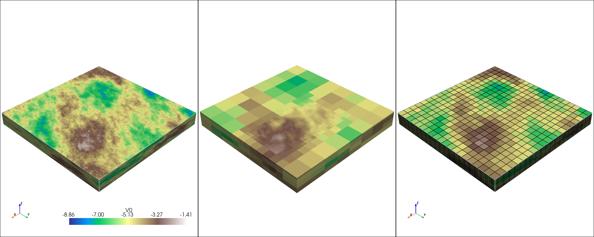
The unstructured upscaled model looks different than reference and structured upscaled model because of the extent that is different. unstructured grid is slightly smaller than the reference grid.

3D DISU
Uppy can also work with DISU grids. As long as the cells of the grid are rectangles, upscaling is possible.
[51]:
# 3D example
# grid dimensions
nlay = 4
nrow = 8
ncol = 8
delr = 100.
delc = 100.
top = 0.
botm = np.linspace(-10, -100, nlay)

sim = flopy.mf6.MFSimulation(
    sim_name="asdf", sim_ws="ws", exe_name="mf6")
tdis = flopy.mf6.ModflowTdis(sim, time_units="DAYS", perioddata=[[1.0, 1, 1.0]])
ms = flopy.mf6.ModflowGwf(sim, modelname="asdf", save_flows=True)
dis = flopy.mf6.ModflowGwfdis(
    ms,
    nlay=nlay,
    nrow=nrow,
    ncol=ncol,
    delr=delr,
    delc=delc,
    top=top,
    botm=botm,
    xorigin=1103.3,
    yorigin=1103.5,
)

# create Gridgen object
g = Gridgen(ms.modelgrid, model_ws="gridgen_ws", exe_name=gridgen_path)

polygon = [
    [
        (1600, 1350),
        (1700, 1300),
        (1300, 1800),
        (1300, 1700),
        (1600, 1350),
    ]
]


g.add_refinement_features([polygon], "polygon", 3, range(1))
refshp0 = "gridgen_ws/" + "rf0"
[52]:
g.build(verbose=False)
[53]:
ms.dis.remove()
# disv_gridprops = g.get_gridprops_disv()
grid_prop_disu = g.get_gridprops_disu6()
# disv = flopy.mf6.ModflowGwfdisv(ms, **disv_gridprops, xorigin=0, yorigin=0)
disu = flopy.mf6.ModflowGwfdisu(ms, **grid_prop_disu, xorigin=0, yorigin=0)
[54]:
# plot a cross section
from flopy.plot import PlotCrossSection

linex, liney = [1100, 1900], [1800, 1400]

mm = flopy.plot.PlotMapView(model=ms)
mm.plot_grid()
plt.plot(linex, liney, "r-")
plt.show()

fig = plt.figure(figsize=(4.8, 3))
xsect = PlotCrossSection(model=ms,geographic_coords=True, line={"line": [linex, liney]})
xsect.plot_grid()
plt.show()
[55]:
grid = ms.modelgrid
[56]:
Kxx, Kyy, Kzz = upscale_k(field, dx=sx_grid, dy=sy_grid, dz=sz_grid, ox=ox_grid, oy=oy_grid, oz=oz_grid, method="simplified_renormalization_C", grid=grid) # upscale the field
[57]:
Kxx = np.log10(Kxx)
Kyy = np.log10(Kyy)
Kzz = np.log10(Kzz)
[58]:
#extract vtk params for plotting with pyvista
vert_exag = 1
vtk = Vtk(model=ms, binary=False, vertical_exageration=vert_exag, smooth=False)
vtk.add_model(ms)
vtk.add_array(Kxx, name="K")
vtk.add_array(Kyy, name="Kyy")
vtk.add_array(Kzz, name="Kzz")
gwf_mesh = vtk.to_pyvista()
[59]:
import pyvista as pv
pv.set_plot_theme("document")
pv.set_jupyter_backend('static')

pl = pv.Plotter(shape=(1, 3), window_size=[2000, 800])
pl.subplot(0, 0)
geone.imgplot3d.drawImage3D_surface(field_img, plotter=pl, cmap="terrain", opacity=1)

pl.subplot(0, 1)
pl.add_mesh(gwf_mesh, opacity=1, scalars="K", cmap="terrain", clim=[field_img.val.min(), field_img.val.max()], show_edges=True)

pl.subplot(0, 2)
arr = field_kxx
arr = np.flipud(np.flip(arr, axis=1))
img = geone.img.Img(nx=arr.shape[2], ny=arr.shape[1], nz=arr.shape[0], sx=sx_grid*10, sy=sy_grid*10, sz=sz_grid*10, ox=0, oy=0, oz=-100, nv=1, val=arr.flatten())
geone.imgplot3d.drawImage3D_surface(img, plotter=pl, cmap="terrain", opacity=1, show_edges=True, cmin=field_img.val.min(), cmax=field_img.val.max())

pl.show()
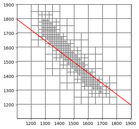
[60]:
# plot a cross section
from flopy.plot import PlotCrossSection
linex, liney = [1100, 1900], [1800, 1200]
mm = flopy.plot.PlotMapView(model=ms)
mm.plot_grid()
plt.plot(linex, liney, "r-")
plt.show()
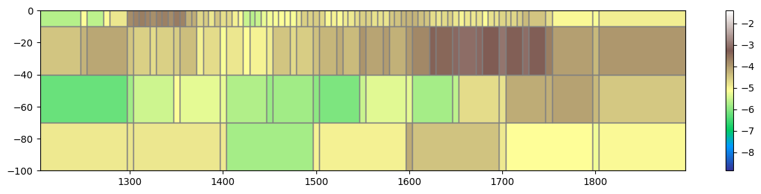
fig = plt.figure(figsize=(15, 3))
xsect = PlotCrossSection(model=ms,geographic_coords=True, line={"line": [linex, liney]})
g = xsect.plot_array(Kxx, alpha=1, cmap="terrain", vmin=field_img.val.min(), vmax=field_img.val.max())
plt.colorbar(g)
xsect.plot_grid()
plt.show()
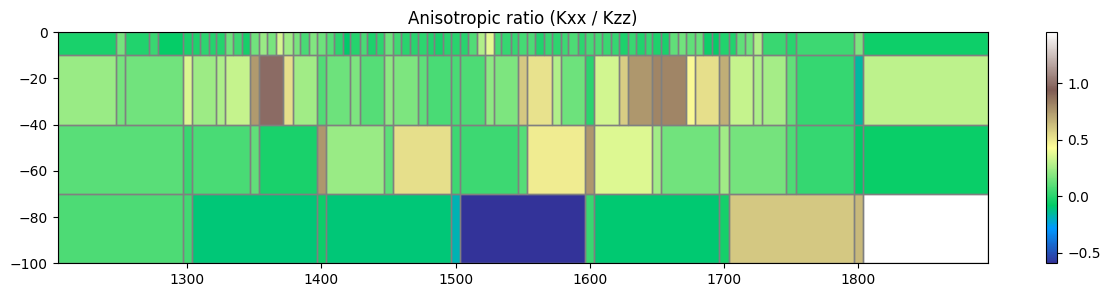
fig = plt.figure(figsize=(15, 3))
xsect = PlotCrossSection(model=ms,geographic_coords=True, line={"line": [linex, liney]})
g = xsect.plot_array(Kxx - Kzz, alpha=1, cmap="terrain")
plt.title("Anisotropic ratio (Kxx / Kzz)")
plt.colorbar(g)
xsect.plot_grid()
plt.show()
[ ]: