Tutorial 2: hard data files

import numpy as np
import matplotlib.pyplot as plt
import geone
import geone.covModel as gcm
import os
import sys
import pyvista as pv
pv.set_jupyter_backend('static')
import pandas as pd

try:
    import ArchPy
except: # if ArchPy is not installed
    print("ArchPy not installed")
    sys.path.append("../..")
    import ArchPy

Introduction

This notebook present how to load and import hard data files (boreholes) with ArchPy.

For this ArchPy requires three different data files which are text files. A list of borholes, a list of unit data and a list of facies data.

They can have any extensions but the recommended are :

list of boreholes -> .lbh

list of unit data -> .ud

list of facies data -> .fd

For this example, the files are in the 2_data_folder.

We can detail these files :

• .lbh : text file with five columns listing all the boreholes in the data. It has five columns and default headers are :

  • bh_ID : borehole identifier to know at which borehole a unit/facies data belongs

  • bh_x : x borehole coordinate

  • bh_y : y borehole coordinate

  • bh_z : z borehole coordinate

  • bh_depth : borehole depth

• .ud : text file with four columns listing all the stratigraphical unit interval data. Default headers are :

  • bh_ID : borehole identifier to know at whcih borehole the unit data belongs

  • Strat : Unit identifier to know at which unit this unit interval data belongs

  • top : top elevation of the interval

  • bot : bot elevation of the interval

• .fd : text file with four columns listing all the facies interval data. Default headers are :

  • bh_ID : borehole identifier to know at whcih borehole the unit data belongs

  • facies_ID : facies identifier to know at which facies this facies interval data belongs

  • top : top elevation of the interval

  • bot : bot elevation of the interval

#path to the files
folder = "2_data_folder"
l_bh_path = pd.read_csv(os.path.join(folder, "IO_exemple.lbh"))

unit_data_path = pd.read_csv(os.path.join(folder, "IO_exemple.ud"))

facies_data_path = pd.read_csv(os.path.join(folder, "IO_exemple.fd"))

First step : import

We can now import the geological database with the function : ArchPy.inputs.load_bh_files

This function takes the dataframe of the 3 inputs files as arguments but also column names if they are differents (e.g. bh_id_col which is by default “bh_ID” or u_top_col which is the name of the column indicating top elevation in .ud file).

Dictionnaries can also be passed (dic_units_names and dic_facies_names) which will change units/facies names in database with associated values in dictionnary. For example, if a dic_units_names = {"Lias" : "Jura",  "Dogger" : "Jura", "Malm" : "Jurassic"} is passed, all unit names in keys will be replaced by “Jurassic”. This can be useful to merge some facies or units if they are similar.

Last parameter is altitude flag which indicates to ArchPy if elevation values in database are in altitude or not (depth if False).

It returns two dataframes : the geological database (db) and the list of boreholes with columns properly renamed to be used in extract_bhs function.

#import data
db, l_bhs = ArchPy.inputs.load_bh_files(list_bhs=l_bh_path,
                            units_data=unit_data_path,
                            facies_data=facies_data_path, altitude=True)
db #print database

	Strat_ID	Facies_ID	top	bot
bh_ID
bh1	B	Clay	15.0	10.0
bh1	B	Sand	10.0	8.0
bh1	B	Clay	8.0	5.0
bh1	A	Silt	5.0	2.0
bh1	A	Gravel	2.0	-1.0
bh1	A	Sand	-1.0	-5.0
bh2	C	Gravel	15.0	10.0
bh2	B	Sand	10.0	8.0
bh2	B	Clay	8.0	4.0
bh2	A	Sand	4.0	2.0
bh2	A	Silt	2.0	-2.0
bh3	C	Gravel	15.0	12.0
bh3	B	Sand	12.0	11.0
bh3	B	Clay	11.0	8.0
bh3	B	Sand	8.0	7.5
bh3	B	Clay	7.5	7.0
bh3	A	Silt	7.0	5.0
bh3	A	Sand	5.0	4.0
bh3	A	Gravel	4.0	2.0
bh3	A	Silt	2.0	0.0

The database has been imported but no project has been defined. We need to create one that respects the Hard data present here.

Second step

Creating the Project with appropriated units/facies.

For simplicity SIS will be used to fill these units.

T1 = ArchPy.base.Arch_table(name = "ex2", working_directory="2_data_folder", seed = 10, verbose = 1)

nx = 150 #number of cells in x
ny = 150
nz = 50
sx = 0.2 #cell width in x
sy = 0.2
sz = 0.5
ox = 0 # x coordinates of the origin
oy = 0
oz = -10
dimensions = (nx, ny, nz)
spacing = (sx, sy, sz)
origin = (ox, oy, oz)

T1.add_grid(dimensions, spacing, origin) #adding the grid

## Adding Grid ##
## Grid added and is now simulation grid ##

P1 = ArchPy.base.Pile("Pile_1")
T1.set_Pile_master(P1)

Pile sets as Pile master

Units

##C
#Creation of the top unit C
covmodel_SIS = gcm.CovModel3D(elem = [("spherical", {"w":2, "r": [20,20,10]}),
                                      ("exponential", {"w":1, "r": [30,30,10]})])

dic_facies_c = {"f_method" : "homogenous", #filling method
                 "f_covmodel" : covmodel_SIS, #SIS covmodels
                } #dictionnary for the unit filling

C = ArchPy.base.Unit(name = "C",
                      order = 1,       #order in pile
                      color = "lightgreen",
                      surface=ArchPy.base.Surface(),  # top surface
                      ID = 1,
                      dic_facies=dic_facies_c
                     )


## B
#surface B
covmodel_b = gcm.CovModel2D(elem = [("cubic", {"w":2, "r" : [15,5]})])
dic_surf_b = {"covmodel" : covmodel_b, "int_method" : "grf_ineq"}
Sb = ArchPy.base.Surface(name = "Sb", dic_surf=dic_surf_b)

#dic facies b
dic_facies_b = {"f_method" : "SIS", "f_covmodel" : covmodel_SIS, "probability" : [0.7, 0.3]}

B = ArchPy.base.Unit(name = "B",
                      order = 2,   #order in pile
                      color = "greenyellow", #color
                      surface=Sb, # top surface
                      ID = 2,     #ID
                      dic_facies=dic_facies_b #facies dictionnary
                     )


##A
covmodel_a = gcm.CovModel2D(elem = [("spherical", {"w":1, "r" : [5,5]})])
dic_surf_a = {"covmodel" : covmodel_b, "int_method" : "grf_ineq"}
Sa = ArchPy.base.Surface(name = "Sa", dic_surf=dic_surf_a)

#dic facies a
dic_facies_a = {"f_method" : "SIS", "f_covmodel" : covmodel_SIS}

A = ArchPy.base.Unit(name = "A",
                      order = 3,   #order in pile
                      color = "lightcoral", #color
                      surface=Sa, # top surface
                      ID = 3,     #ID
                      dic_facies=dic_facies_a #facies dictionnary
                     )

#Adding the units to the Pile
P1.add_unit([C, B, A])

Unit C: Surface added for interpolation
Unit B: covmodel for SIS added
Unit B: Surface added for interpolation
Unit A: covmodel for SIS added
Unit A: Surface added for interpolation
Stratigraphic unit C added ✅
Stratigraphic unit B added ✅
Stratigraphic unit A added ✅

Facies

Sand = ArchPy.base.Facies(ID = 1, name = "Sand", color = "yellow")
Clay = ArchPy.base.Facies(ID = 2, name = "Clay", color = "royalblue")
Gravel = ArchPy.base.Facies(ID = 3, name = "Gravel", color = "palegreen")
Silt = ArchPy.base.Facies(ID = 4, name = "Silt", color = "goldenrod")


C.add_facies(Gravel)
B.add_facies([Clay, Sand])
A.add_facies([Sand, Gravel, Silt])

Facies Gravel added to unit C ✅
Facies Clay added to unit B ✅
Facies Sand added to unit B ✅
Facies Sand added to unit A ✅
Facies Gravel added to unit A ✅
Facies Silt added to unit A ✅

Extract boreholes from database

We can now extract boreholes objects with ArchPy.inputs.extract_bhs. Note : This function requires the list of boreholes path

boreholes = ArchPy.inputs.extract_bhs(df=db, list_bhs=l_bhs, ArchTable=T1)

Borehole class

In ArchPy, the geological data are in “borehole” format. Here we have created boreholes directly from a database but they can also be create manually in python with ArchPy.base.borehole.

A borehole takes multiple arguments :

• name

• ID

• x,y,z : top borehole coordinates

• depth : depth of the borehole

• log_strati : unit data which is a list of tuple, each tuple containing a unit object and an elevation (e.g. log_strati = [(D, 10), (C, 6), ...]).

• log_facies : facies data, identical to log_strati except unit object are facies object

They are added to the project with add_bh.

T1.add_bh(boreholes)

Borehole bh1 added
Borehole bh2 added
Borehole bh3 added

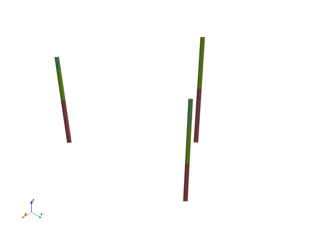
#We can look at what the boreholes looks with plot_bhs()
p=pv.Plotter()
T1.plot_bhs(plotter=p)
p.show_axes()
p.show()

It is now important to process the data in order to get the HD correctly

All this step is automated by calling process_bhs

T1.process_bhs()

##### ORDERING UNITS #####
Pile Pile_1: ordering units
Stratigraphic units have been sorted according to order
hierarchical relations set

 ## Computing distributions for Normal Score Transform ##

Processing ended successfully

Check

We can check that Hard Data have been extracted. They are stored inside surface objects directly. Here with B top surface that have 2 equality point and 1 inequality point (lower boundary)

unit = B

for ix,iy,iz in zip(unit.surface.x,unit.surface.y,unit.surface.z):
    print("equality point : {} x, {} y, {} z".format(ix,iy,iz))

for ineq in unit.surface.ineq:
    print("inequality point : {} x, {} y, {} vmin, {} vmax".format(ineq[0], ineq[1], ineq[3], ineq[4]))

equality point : 15 x, 25 y, 10.0 z
equality point : 20 x, 5 y, 12.0 z
inequality point : 1 x, 15 y, 14.0 vmin, nan vmax

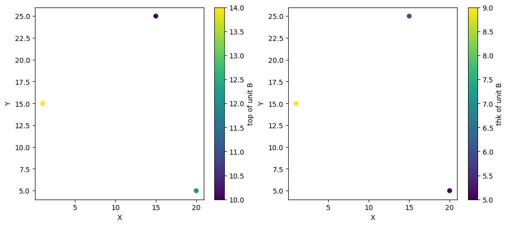
We can also plot on a top-view the hard data

plt.figure(figsize=(12,5))
plt.subplot(1, 2, 1)
T1.plot_unit_data_point(B)
plt.subplot(1, 2, 2)
T1.plot_unit_data_point(B, typ="thk")

Simulations

T1.compute_surf(1)

########## PILE Pile_1 ##########
Pile Pile_1: ordering units
Stratigraphic units have been sorted according to order

#### COMPUTING SURFACE OF UNIT A
A: time elapsed for computing surface 0.03850197792053223 s

#### COMPUTING SURFACE OF UNIT B
B: time elapsed for computing surface 0.03570961952209473 s

#### COMPUTING SURFACE OF UNIT C
C: time elapsed for computing surface 0.0 s

Time elapsed for getting domains 0.009617328643798828 s
##########################


### 0.10334396362304688: Total time elapsed for computing surfaces ###

T1.compute_facies(1)

### Unit C: facies simulation with homogenous method ####
### Unit C - realization 0 ###
Time elapsed 0.0 s

### Unit B: facies simulation with SIS method ####
### Unit B - realization 0 ###
Only one facies covmodels for multiples facies, adapt sill to right proportions
Time elapsed 1.59 s

### Unit A: facies simulation with SIS method ####
### Unit A - realization 0 ###
Only one facies covmodels for multiples facies, adapt sill to right proportions
Time elapsed 3.12 s

### 4.72: Total time elapsed for computing facies ###

p = pv.Plotter()

v_ex = 1
T1.plot_units(plotter=p, slicex=(0.5), slicey=(0.5),v_ex=v_ex)
T1.plot_bhs(plotter=p, v_ex=v_ex)
p.show()

p = pv.Plotter()
T1.plot_facies(plotter=p, slicex=(0.5), slicey=(0.5),v_ex=1)
T1.plot_bhs("facies", plotter=p, v_ex=1)
p.show()

This concludes this little tutorial on ArchPy inputs capabilities