Modflow/Modpath basics
[1]:
import numpy as np
import pandas as pd
import matplotlib
from matplotlib import colors
import matplotlib.pyplot as plt
import geone
import geone.covModel as gcm
import geone.imgplot3d as imgplt3
import pyvista as pv
import sys
import os

# auto reload modules
%load_ext autoreload
%autoreload 2


sys.path.append("../../")
#my modules
from ArchPy.base import *
from ArchPy.tpgs import *
[2]:
#grid
sx = 1.5
sy = 1.5
sz = .15
x0 = 0
y0 = 0
z0 = -15
nx = 140
ny = 70
nz = 70
x1 = x0 + nx*sx
y1 = y0 + ny*sy
z1 = z0 + nz

dimensions = (nx, ny, nz)
spacing = (sx, sy, sz)
origin = (x0, y0, z0)
[3]:
## create pile

P1 = Pile(name = "P1",seed=1)

#units covmodel
covmodelD = gcm.CovModel2D(elem=[('cubic', {'w':0.6, 'r':[30,30]})])
covmodelD1 = gcm.CovModel2D(elem=[('cubic', {'w':0.2, 'r':[30,30]})])
covmodelC = gcm.CovModel2D(elem=[('cubic', {'w':0.2, 'r':[40,40]})])
covmodelB = gcm.CovModel2D(elem=[('cubic', {'w':0.6, 'r':[30,30]})])
covmodel_er = gcm.CovModel2D(elem=[('spherical', {'w':1, 'r':[50,50]})])

## facies covmodel
covmodel_SIS_C = gcm.CovModel3D(elem=[("exponential", {"w":.21,"r":[50, 50, 10]})], alpha=0, name="vario_SIS") # input variogram
covmodel_SIS_B1 = gcm.CovModel3D(elem=[("exponential", {"w":.16,"r":[50, 50, 2]})], alpha=0, name="vario_SIS") # input variogram
covmodel_SIS_B2 = gcm.CovModel3D(elem=[("exponential", {"w":.24,"r":[100, 100, 3]})], alpha=0, name="vario_SIS") # input variogram
covmodel_SIS_B3 = gcm.CovModel3D(elem=[("exponential", {"w":.19,"r":[50, 50, 2]})], alpha=0, name="vario_SIS") # input variogram
covmodel_SIS_B4 = gcm.CovModel3D(elem=[("exponential", {"w":.13,"r":[100, 100, 4]})], alpha=0, name="vario_SIS") # input variogram

lst_covmodelC=[covmodel_SIS_C] # list of covmodels to pass at the function
lst_covmodelB=[covmodel_SIS_B1, covmodel_SIS_B2, covmodel_SIS_B3, covmodel_SIS_B4] # list of covmodels to pass


#create Lithologies
dic_s_D = {"int_method" : "grf_ineq","covmodel" : covmodelD}
dic_f_D = {"f_method":"homogenous"}
D = Unit(name="D",order=1,ID = 1,color="gold",contact="onlap",surface=Surface(contact="onlap",dic_surf=dic_s_D)
         ,dic_facies=dic_f_D)

dic_s_C = {"int_method" : "grf_ineq","covmodel" : covmodelC, "mean":-6.5}
dic_f_C = {"f_method" : "SIS","neig" : 10, "f_covmodel":lst_covmodelC, "probability":[0.3, 0.7]}
C = Unit(name="C", order=2, ID = 2, color="blue", contact="onlap", dic_facies=dic_f_C, surface=Surface(dic_surf=dic_s_C, contact="onlap"))

dic_s_B = {"int_method" : "grf_ineq","covmodel" : covmodelB, "mean":-8.5}
dic_f_B = {"f_method":"SIS", "neig" : 10, "f_covmodel":lst_covmodelB, "probability":[0.2, 0.4, 0.25, 0.15]}
B = Unit(name="B",order=3,ID = 3,color="purple",contact="onlap",dic_facies=dic_f_B,surface=Surface(contact="onlap",dic_surf=dic_s_B))

dic_s_A = {"int_method":"grf_ineq","covmodel": covmodelB, "mean":-11}
dic_f_A = {"f_method":"homogenous"}
A = Unit(name="A",order=5,ID = 5,color="red",contact="onlap",dic_facies=dic_f_A,surface=Surface(dic_surf = dic_s_A,contact="onlap"))

#Master pile
P1.add_unit([D,C,B,A])
Unit D: Surface added for interpolation
Unit C: Surface added for interpolation
Unit B: Surface added for interpolation
Unit A: Surface added for interpolation
Stratigraphic unit D added ✅
Stratigraphic unit C added ✅
Stratigraphic unit B added ✅
Stratigraphic unit A added ✅
[4]:
# covmodels for the property model
covmodelK = gcm.CovModel3D(elem=[("exponential",{"w":0.3,"r":[30,30,10]})],alpha=-20,name="K_vario")
covmodelK2 = gcm.CovModel3D(elem=[("spherical",{"w":0.1,"r":[20,20, 5]})],alpha=0,name="K_vario_2")

facies_1 = Facies(ID = 1,name="Sand",color="yellow")
facies_2 = Facies(ID = 2,name="Gravel",color="lightgreen")
facies_3 = Facies(ID = 3,name="GM",color="blueviolet")
facies_4 = Facies(ID = 4,name="Clay",color="blue")
facies_5 = Facies(ID = 5,name="SM",color="brown")
facies_6 = Facies(ID = 6,name="Silt",color="goldenrod")
facies_7 = Facies(ID = 7,name="basement",color="red")

A.add_facies([facies_7])
B.add_facies([facies_1, facies_2, facies_3, facies_5])
D.add_facies([facies_1])
C.add_facies([facies_4, facies_6])

# property model
cm_prop1 = gcm.CovModel3D(elem = [("spherical", {"w":0.1, "r":[10,10,10]}),
                                  ("cubic", {"w":0.1, "r":[15,15,15]})])
cm_prop2 = gcm.CovModel3D(elem = [("cubic", {"w":0.2, "r":[25, 25, 5]})])

list_facies = [facies_1, facies_2, facies_3, facies_4, facies_5, facies_6, facies_7]
list_covmodels = [cm_prop2, cm_prop1, cm_prop2, cm_prop1, cm_prop2, cm_prop1, cm_prop2]
means = [-4, -2, -6, -9, -6, -7, -19]
prop_model = ArchPy.base.Prop("K",
                              facies = list_facies,
                              covmodels = list_covmodels,
                                means = means,
                                int_method = "sgs",
                                vmin = -10,
                                vmax = -1
                                )
Facies basement added to unit A ✅
Facies Sand added to unit B ✅
Facies Gravel added to unit B ✅
Facies GM added to unit B ✅
Facies SM added to unit B ✅
Facies Sand added to unit D ✅
Facies Clay added to unit C ✅
Facies Silt added to unit C ✅
[5]:
top = np.ones([ny,nx])*-6
bot = np.ones([ny,nx])*z0
[6]:
T1 = Arch_table(name = "P1",seed=3)
T1.set_Pile_master(P1)
T1.add_grid(dimensions, spacing, origin, top=top,bot=bot)
T1.add_prop(prop_model)
Pile sets as Pile master
## Adding Grid ##
## Grid added and is now simulation grid ##
Property K added
[7]:
T1.compute_surf(1)
T1.compute_facies(1)
T1.compute_prop(1)
Boreholes not processed, fully unconditional simulations will be tempted
########## PILE P1 ##########
Pile P1: ordering units
Stratigraphic units have been sorted according to order
Discrepency in the orders for units A and B
Changing orders for that they range from 1 to n

#### COMPUTING SURFACE OF UNIT A
A: time elapsed for computing surface 0.01258087158203125 s

#### COMPUTING SURFACE OF UNIT B
B: time elapsed for computing surface 0.011628389358520508 s

#### COMPUTING SURFACE OF UNIT C
C: time elapsed for computing surface 0.012747526168823242 s

#### COMPUTING SURFACE OF UNIT D
D: time elapsed for computing surface 0.0 s

Time elapsed for getting domains 0.0060350894927978516 s
##########################


### 0.060006141662597656: Total time elapsed for computing surfaces ###

### Unit D: facies simulation with homogenous method ####
### Unit D - realization 0 ###
Time elapsed 0.0 s

### Unit C: facies simulation with SIS method ####
### Unit C - realization 0 ###
Only one facies covmodels for multiples facies, adapt sill to right proportions
Time elapsed 0.39 s

### Unit B: facies simulation with SIS method ####
### Unit B - realization 0 ###
Time elapsed 0.69 s

### Unit A: facies simulation with homogenous method ####
### Unit A - realization 0 ###
Time elapsed 0.0 s

### 1.08: Total time elapsed for computing facies ###
### 1 K property models will be modeled ###
### 1 K models done
[8]:
import flopy as fp
[9]:
pv.set_jupyter_backend("static")
[10]:
T1.plot_units(v_ex=3)

[11]:
T1.plot_facies(v_ex=3)

[12]:
T1.plot_prop("K", v_ex=3)

[13]:
val = T1.get_prop("K")[0, 0, 0]
im = geone.img.Img(nx=nx, ny=ny, nz=nz, sx=sx, sy=sy, sz=sz, ox=x0, oy=y0, oz=z0, nv=1, val=val)
[14]:
factor_x = 4
factor_y = 2
factor_z = 2

nlay, nrow, ncol = T1.get_nz(), T1.get_ny(), T1.get_nx()
delr, delc = T1.get_sx(), T1.get_sy()
xoff, yoff = T1.get_ox(), T1.get_oy()

assert factor_x is not None, "factor_x must be provided"
assert factor_y is not None, "factor_y must be provided"
assert factor_z is not None, "factor_z must be provided"
assert nrow % factor_y == 0, "nrow must be divisible by factor_y"
assert ncol % factor_x == 0, "ncol must be divisible by factor_x"
assert nlay % factor_z == 0, "nlay must be divisible by factor_z"
nrow = int(nrow / factor_y)
ncol = int(ncol / factor_x)
nlay = int(nlay / factor_z)
delr = delr * factor_x
delc = delc * factor_y
top = np.ones((nrow, ncol)) * T1.get_zg()[-1]
botm = np.ones((nlay, nrow, ncol)) * T1.get_zg()[::-factor_z][1:].reshape(-1, 1, 1)
botm = np.flip(np.flipud(botm), axis=1)  # flip the array to have the same orientation as the ArchPy table
botm.shape
[14]:
(35, 35, 35)
[15]:
delc, delr
[15]:
(3.0, 6.0)
archpy2modflow
Here is a simple example of how to use the archpy2modflow package to convert an ArchPy model to a MODFLOW model using the flopy package. Several modes can be used to convert the ArchPy model (and grid) to a MODFLOW model (grid). The modes are:
archpymode: This mode uses the ArchPy grid to create a MODFLOW DIS grid.layersmode: This mode considers that each stratigraphic unit is a modflow layer and uses the surfaces simulated by ArchPy to define the bottom elevation of each layer. K values are averaged between the top and bottom of each layer.new_resolutionmode: upscaled model using the uppy package. New resolution is defined as a factor of reduction in each direction. For example, if the factor in x direction is 2, the new model will have half the number of cells in the x direction, while the number of cells in the y and z directions will remain the same.
Now imagine that you want to set one or several units as inactive in the MODFLOW model (e.g., bedrock, impervious bottom), you can set this with the unit_limit parameter of the create_sim method. This parameter takes a unit name as input and will consider itself and all units below it as inactive.
```python
[16]:
import ArchPy.ap_mf
from ArchPy.ap_mf import archpy2modflow, array2cellids
Let us create our modflow model.
Modflow model
ArchPy mode
[17]:
archpy_flow = archpy2modflow(T1, exe_name="../../../../exe/mf6.exe")  # create the modflow model
archpy_flow.create_sim(grid_mode="archpy", iu=0, unit_limit="A")  # create the simulation object and choose a certain discretization
archpy_flow.set_k("K", iu=0, ifa=0, ip=0, log=True, average_facies=True)  # set the hydraulic conductivity
Simulation created with the following parameters:
Grid mode: archpy
To retrieve the simulation, use the get_sim() method
Here we have instantiate a modflow model based on the ArchPy model and using the same grid resolution. The model is created using the archpy mode. We have also set the npf package to use the K values from the ArchPy model. As ArchPy is a stochastic model we have multiple realization, here it is the one that corresponds to iu=0, ifa=0 and ip=0. We also indicate that K values are in log10 scale.
Now we can retrieve flopy/modflow model and add different packages as we would do with a regular modflow model.
[18]:
sim = archpy_flow.get_sim()
gwf = archpy_flow.get_gwf()
For example some boundary conditions
[19]:
# add BC at left and right on all layers
h1 = 10
h2 = 0
chd_data = []

a = np.zeros((gwf.modelgrid.nlay, gwf.modelgrid.nrow, gwf.modelgrid.ncol), dtype=bool)
a[:, :, 0] = 1
lst_chd = array2cellids(a, gwf.dis.idomain.array)
for cellid in lst_chd:
    chd_data.append((cellid, h1))

a = np.zeros((gwf.modelgrid.nlay, gwf.modelgrid.nrow, gwf.modelgrid.ncol), dtype=bool)
a[:, :, -1] = 1
lst_chd = array2cellids(a, gwf.dis.idomain.array)
for cellid in lst_chd:
    chd_data.append((cellid, h2))

chd = fp.mf6.ModflowGwfchd(gwf, stress_period_data=chd_data, save_flows=True)
[20]:
# modify ims to a more strict convergence criteria
sim.ims.remove()
inner_dvclose = 1e-4
ims = fp.mf6.ModflowIms(sim, complexity="moderate", inner_dvclose=inner_dvclose)

# set IC to help the model converge
dis = gwf.get_package("DIS")
ny, nx, nz = dis.nrow.get_data(), dis.ncol.get_data(), dis.nlay.get_data()
strt = np.linspace(10, 0, nx)
strt = np.tile(strt, (ny, 1))
strt = np.tile(strt, (nz, 1, 1))

archpy_flow.set_strt(strt)
Write modflow model files
[21]:
sim.write_simulation()
writing simulation...
  writing simulation name file...
  writing simulation tdis package...
  writing solution package ims_-1...
  writing model test...
    writing model name file...
    writing package dis...
    writing package oc...
    writing package npf...
    writing package chd_0...
INFORMATION: maxbound in ('', 'chd', 'dimensions') changed to 4666 based on size of stress_period_data
    writing package ic...
Here we also modify the solver to an higher complexity as the model contains a large number of cells and have difficult to converge.
[22]:
sim.run_simulation()
FloPy is using the following executable to run the model: \\home\schorppl$\exe\mf6.exe
                                   MODFLOW 6
                U.S. GEOLOGICAL SURVEY MODULAR HYDROLOGIC MODEL
                            VERSION 6.7.0 02/05/2026

   MODFLOW 6 compiled Feb 05 2026 22:36:44 with Intel(R) Fortran Intel(R) 64
   Compiler Classic for applications running on Intel(R) 64, Version 2021.6.0
                             Build 20220226_000000

This software has been approved for release by the U.S. Geological
Survey (USGS). Although the software has been subjected to rigorous
review, the USGS reserves the right to update the software as needed
pursuant to further analysis and review. No warranty, expressed or
implied, is made by the USGS or the U.S. Government as to the
functionality of the software and related material nor shall the
fact of release constitute any such warranty. Furthermore, the
software is released on condition that neither the USGS nor the U.S.
Government shall be held liable for any damages resulting from its
authorized or unauthorized use. Also refer to the USGS Water
Resources Software User Rights Notice for complete use, copyright,
and distribution information.


 MODFLOW runs in SEQUENTIAL mode

 Run start date and time (yyyy/mm/dd hh:mm:ss): 2026/04/01 10:38:32

 Writing simulation list file: mfsim.lst
 Using Simulation name file: mfsim.nam

    Solving:  Stress period:     1    Time step:     1

 Run end date and time (yyyy/mm/dd hh:mm:ss): 2026/04/01 10:39:09
 Elapsed run time: 36.378 Seconds

 Normal termination of simulation.
[22]:
(True, [])
Now we can retrieve some results. Archpy2modflow objects integrate some basic functions to facilitate this such as get_heads methods.
[23]:
heads = archpy_flow.get_heads(kstpkper=(0, 0))
heads[heads == 1e30] = np.nan
[24]:
cobj = gwf.output.budget()
qx, qy, qz = fp.utils.postprocessing.get_specific_discharge(
        cobj.get_data(text="DATA-SPDIS", kstpkper=(0, 0))[0], gwf)
[25]:
import flopy
from flopy.plot import PlotMapView
mapview = PlotMapView(model=gwf, layer=15)
quadmesh = mapview.plot_array(heads, cmap="Blues")
# quadmesh = mapview.contour_array(heads, cmap="jet", levels=10)
# quadmesh = mapview.plot_array(np.log10(gwf.npf.k.array), cmap="viridis")
mapview.plot_vector(qx, qy, color="black", istep=3, jstep=3)
[25]:
<matplotlib.quiver.Quiver at 0x1f07fe45310>

Be aware that grids between modflow and archpy are not the same. The origin of the grid is at the lowest layer, left and bottom of the model in archpy and at the uppest layer, left and top of the model in modflow (see the figure)

If you have a modflow output and want to plot it in 3D using archpy, you need to flip this array using the following command:
heads = np.flipud(np.flip(heads, axis=1))
If we make a plot of the resulting model, we see that unit A, the bedrock, has been set as inactive in the model.
[26]:
heads = archpy_flow.get_heads()
heads[heads == 1e30] = np.nan

T1.plot_arr(np.flipud(np.flip(heads, axis=1)), "head", 2)

[27]:
T1.plot_prop("K", v_ex=2)

Particle tracking
Modpath simulations
archpy2modflow also integrates function to run modpath simulations. Here is an example of how to run a modpath simulation. Note that it only works with modpath 7.
First we need to create a modpath model and provide the path to the modpath executable. This is done using mp_create method as shown below
Initial starting point of particles can be either defined by a list of coordinates or by a list of cell indices. Here we use the first option and we provide a list to list_p_coord. The tracking direction is also defined by the user. Here we use the backward tracking direction.
[28]:
import ArchPy
[29]:
mpexe_path = "../../../../exe/mp7.exe"
archpy_flow.mp_create(mpexe=mpexe_path,
                      trackdir="backward",
                      list_p_coords=[(170.7, 99.75, -7), (170.7, 99.75, -9)])
C:\Users\schorppl\.conda\envs\archpy\Lib\site-packages\flopy\utils\gridintersect.py:290: DeprecationWarning: In the future this function will return a GeoDataFrame by default. Set geo_dataframe=True to adopt future behavior and silence this warning. Set geo_dataframe=False to silence this warning and maintain old behavior
  warnings.warn(
[30]:
archpy_flow.mp_run(silent=False)
FloPy is using the following executable to run the model: \\home\schorppl$\exe\mp7.exe

MODPATH Version 7.2.002 PROVISIONAL
Program compiled Oct 16 2023 03:40:46 with IFORT compiler (ver. 20.21.7)


Run particle tracking simulation ...
Processing Time Step     1 Period     1.  Time =  1.00000E+00  Steady-state flow

Particle Summary:
         0 particles are pending release.
         0 particles remain active.
         0 particles terminated at boundary faces.
         0 particles terminated at weak sink cells.
         0 particles terminated at weak source cells.
         2 particles terminated at strong source/sink cells.
         0 particles terminated in cells with a specified zone number.
         0 particles were stranded in inactive or dry cells.
         0 particles were unreleased.
         0 particles have an unknown status.

Normal termination.
Pathlines and endpoints objects can be retrieve using archpy2modflow functions
[31]:
p = archpy_flow.mp_get_pathlines_object()
e = archpy_flow.mp_get_endpoints_object()
[32]:
fig = plt.figure(figsize=(10, 10))
path = p.get_alldata()

# 3D plot of the pathlines
fig = plt.figure(figsize=(10, 10))
ax = fig.add_subplot(111, projection="3d")

for pth in path:
    ax.plot(pth["x"], pth["y"], pth["z"])

plt.xlim(0, 200)
plt.ylim(0, 100)
ax.set_zlim(-15, 0)
ax.set_aspect("equal")
plt.show()
<Figure size 1000x1000 with 0 Axes>

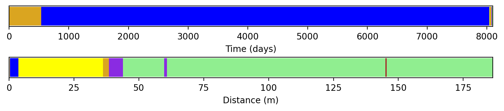
If we want to investigate the encountered lithologies along the pathlines we can use the following command:
archpy_flow.mp_get_facies_path_particle(i_particle)
where i_particle is the index of the particle we want to investigate.
[33]:
from ArchPy.ap_mf import plot_particle_facies_sequence

df = archpy_flow.mp_get_facies_path_particle(1)  # get the facies sequence of the particles
plot_particle_facies_sequence(T1, df, plot_time=True, plot_distance=True)  # plot facies sequences in time and distance

PRT
It can be noted that particle tracking with archpy2modflow can also be done using PRT model from Modflow 6 using similar functions
[34]:
archpy_flow.prt_create(prt_name="test_prt", workspace="ws_prt", trackdir="backward", list_p_coords=[(170.7, 99.75, -7), (170.7, 99.75, -9)])
archpy_flow.prt_run(silent=False)
C:\Users\schorppl\.conda\envs\archpy\Lib\site-packages\flopy\utils\gridintersect.py:290: DeprecationWarning: In the future this function will return a GeoDataFrame by default. Set geo_dataframe=True to adopt future behavior and silence this warning. Set geo_dataframe=False to silence this warning and maintain old behavior
  warnings.warn(
writing simulation...
  writing simulation name file...
  writing simulation tdis package...
  writing solution package ems...
  writing model test_prt...
    writing model name file...
    writing package mip...
    writing package dis...
    writing package prp...
    writing package oc...
    writing package fmi...
FloPy is using the following executable to run the model: \\home\schorppl$\exe\mf6.exe
                                   MODFLOW 6
                U.S. GEOLOGICAL SURVEY MODULAR HYDROLOGIC MODEL
                            VERSION 6.7.0 02/05/2026

   MODFLOW 6 compiled Feb 05 2026 22:36:44 with Intel(R) Fortran Intel(R) 64
   Compiler Classic for applications running on Intel(R) 64, Version 2021.6.0
                             Build 20220226_000000

This software has been approved for release by the U.S. Geological
Survey (USGS). Although the software has been subjected to rigorous
review, the USGS reserves the right to update the software as needed
pursuant to further analysis and review. No warranty, expressed or
implied, is made by the USGS or the U.S. Government as to the
functionality of the software and related material nor shall the
fact of release constitute any such warranty. Furthermore, the
software is released on condition that neither the USGS nor the U.S.
Government shall be held liable for any damages resulting from its
authorized or unauthorized use. Also refer to the USGS Water
Resources Software User Rights Notice for complete use, copyright,
and distribution information.


 MODFLOW runs in SEQUENTIAL mode

 Run start date and time (yyyy/mm/dd hh:mm:ss): 2026/04/01 10:39:20

 Writing simulation list file: mfsim.lst
 Using Simulation name file: mfsim.nam

    Solving:  Stress period:     1    Time step:     1

 Run end date and time (yyyy/mm/dd hh:mm:ss): 2026/04/01 10:39:21
 Elapsed run time:  0.983 Seconds

 Normal termination of simulation.
[35]:
fig = plt.figure(figsize=(10, 10))

# 3D plot of the pathlines
fig = plt.figure(figsize=(10, 10))
ax = fig.add_subplot(111, projection="3d")

for i in range(3):
    path = archpy_flow.prt_get_pathlines(i_particle=i+1)
    plt.plot(path["x"], path["y"], path["z"])

plt.xlim(0, 200)
plt.ylim(0, 100)
ax.set_zlim(-15, 0)
ax.set_aspect("equal")
plt.show()
<Figure size 1000x1000 with 0 Axes>

[36]:
df_prt = archpy_flow.prt_get_facies_path_particle(2)  # get the facies sequence of the particles
ArchPy.ap_mf.plot_particle_facies_sequence(T1, df_prt, plot_time=True, plot_distance=True)  # plot facies sequences in time and distance
Layers mode
Now investigate the layer mode where each archpy unit is now a modflow layer. K values are then averaged to give the mean K values in each cell of the layer. Several averages are available. anisotropic average performs an arithmetic mean to obtain Kxx and Kyy while Kzz is the harmonic mean of the K values in the layer.
The lay_sep is a list of int indicating the number of layers that should be created for each archpy unit. Here only third unit is separated into 3 layers.
surface_layer=True allows to create a superficial layer with a thickness defined by surface_thickness at the top of the model. This additional surface has same properties than the layer below it (ex- first layer).
[37]:
import ArchPy
[38]:
archpy_flow = archpy2modflow(T1, exe_name="../../../../exe/mf6.exe")
archpy_flow.create_sim(grid_mode="layers", iu=0, unit_limit="A", lay_sep=[1, 2, 3, 1], surface_layer=True)
Simulation created with the following parameters:
Grid mode: layers
To retrieve the simulation, use the get_sim() method
[39]:
archpy_flow.set_k(k_key="K", iu=0, ifa=0, ip=0, log=True, k_average_method="anisotropic", average_facies=True, surface_k=10**-4)
[40]:
sim = archpy_flow.get_sim()
gwf = archpy_flow.get_gwf()
[41]:
plt.imshow(np.log10(gwf.npf.k.array[:, 45]), aspect=3)
[41]:
<matplotlib.image.AxesImage at 0x1f0b401bc90>
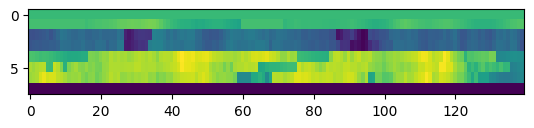
Plot to check the grid
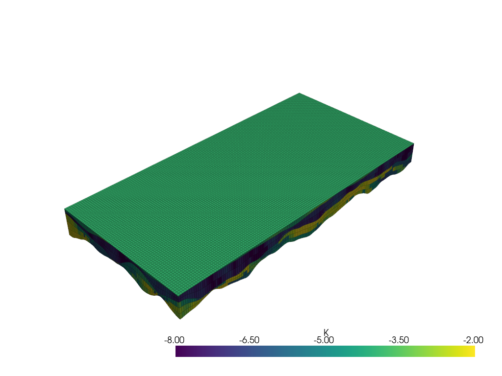
[42]:
from flopy.export.vtk import Vtk

vert_exag = 3
vtk = Vtk(model=gwf, binary=False, vertical_exageration=vert_exag, smooth=True)
vtk.add_model(gwf)

vtk.add_array(np.log10(gwf.npf.k.array), name="K")
vtk.add_array(gwf.npf.k.array / gwf.npf.k33.array, name="K_anisotropy")
gwf_mesh = vtk.to_pyvista()

ghosts = np.argwhere(gwf_mesh["idomain"] == 0)
gwf_mesh.remove_cells(ghosts, inplace=True)

pl = pv.Plotter(notebook=True)
pl.add_mesh(gwf_mesh, opacity=1, show_edges=True, scalars="K", cmap="viridis", clim=[-8, -2], edge_opacity=0.3)
pl.show()
[43]:
pl = pv.Plotter(notebook=True)
pl.add_mesh(gwf_mesh, opacity=1, show_edges=True, scalars="K_anisotropy", cmap="viridis", clim=[0, 100], edge_opacity=0.3)
pl.show()

[44]:
# add BC at left and right on all layers
h1 = 10
h2 = 0
chd_data = []

a = np.zeros((gwf.modelgrid.nlay, gwf.modelgrid.nrow, gwf.modelgrid.ncol), dtype=bool)
a[:, :, 0] = 1
lst_chd = array2cellids(a, gwf.dis.idomain.array)
for cellid in lst_chd:
    chd_data.append((cellid, h1))

a = np.zeros((gwf.modelgrid.nlay, gwf.modelgrid.nrow, gwf.modelgrid.ncol), dtype=bool)
a[:, :, -1] = 1
lst_chd = array2cellids(a, gwf.dis.idomain.array)
for cellid in lst_chd:
    chd_data.append((cellid, h2))

chd = fp.mf6.ModflowGwfchd(gwf, stress_period_data=chd_data, save_flows=True)
[45]:
sim.write_simulation()
sim.ims.complexity = "moderate"
sim.ims.write()
sim.run_simulation()
writing simulation...
  writing simulation name file...
  writing simulation tdis package...
  writing solution package ims_-1...
  writing model test...
    writing model name file...
    writing package dis...
    writing package ic...
    writing package oc...
    writing package npf...
    writing package chd_0...
INFORMATION: maxbound in ('', 'chd', 'dimensions') changed to 953 based on size of stress_period_data
FloPy is using the following executable to run the model: \\home\schorppl$\exe\mf6.exe
                                   MODFLOW 6
                U.S. GEOLOGICAL SURVEY MODULAR HYDROLOGIC MODEL
                            VERSION 6.7.0 02/05/2026

   MODFLOW 6 compiled Feb 05 2026 22:36:44 with Intel(R) Fortran Intel(R) 64
   Compiler Classic for applications running on Intel(R) 64, Version 2021.6.0
                             Build 20220226_000000

This software has been approved for release by the U.S. Geological
Survey (USGS). Although the software has been subjected to rigorous
review, the USGS reserves the right to update the software as needed
pursuant to further analysis and review. No warranty, expressed or
implied, is made by the USGS or the U.S. Government as to the
functionality of the software and related material nor shall the
fact of release constitute any such warranty. Furthermore, the
software is released on condition that neither the USGS nor the U.S.
Government shall be held liable for any damages resulting from its
authorized or unauthorized use. Also refer to the USGS Water
Resources Software User Rights Notice for complete use, copyright,
and distribution information.


 MODFLOW runs in SEQUENTIAL mode

 Run start date and time (yyyy/mm/dd hh:mm:ss): 2026/04/01 10:39:28

 Writing simulation list file: mfsim.lst
 Using Simulation name file: mfsim.nam

    Solving:  Stress period:     1    Time step:     1

 Run end date and time (yyyy/mm/dd hh:mm:ss): 2026/04/01 10:39:29
 Elapsed run time:  1.107 Seconds

 Normal termination of simulation.
[45]:
(True, [])
[46]:
heads = archpy_flow.get_heads()
heads[heads == 1e30] = np.nan

cobj = gwf.output.budget()
qx, qy, qz = fp.utils.postprocessing.get_specific_discharge(
        cobj.get_data(text="DATA-SPDIS", kstpkper=(0, 0))[0], gwf)
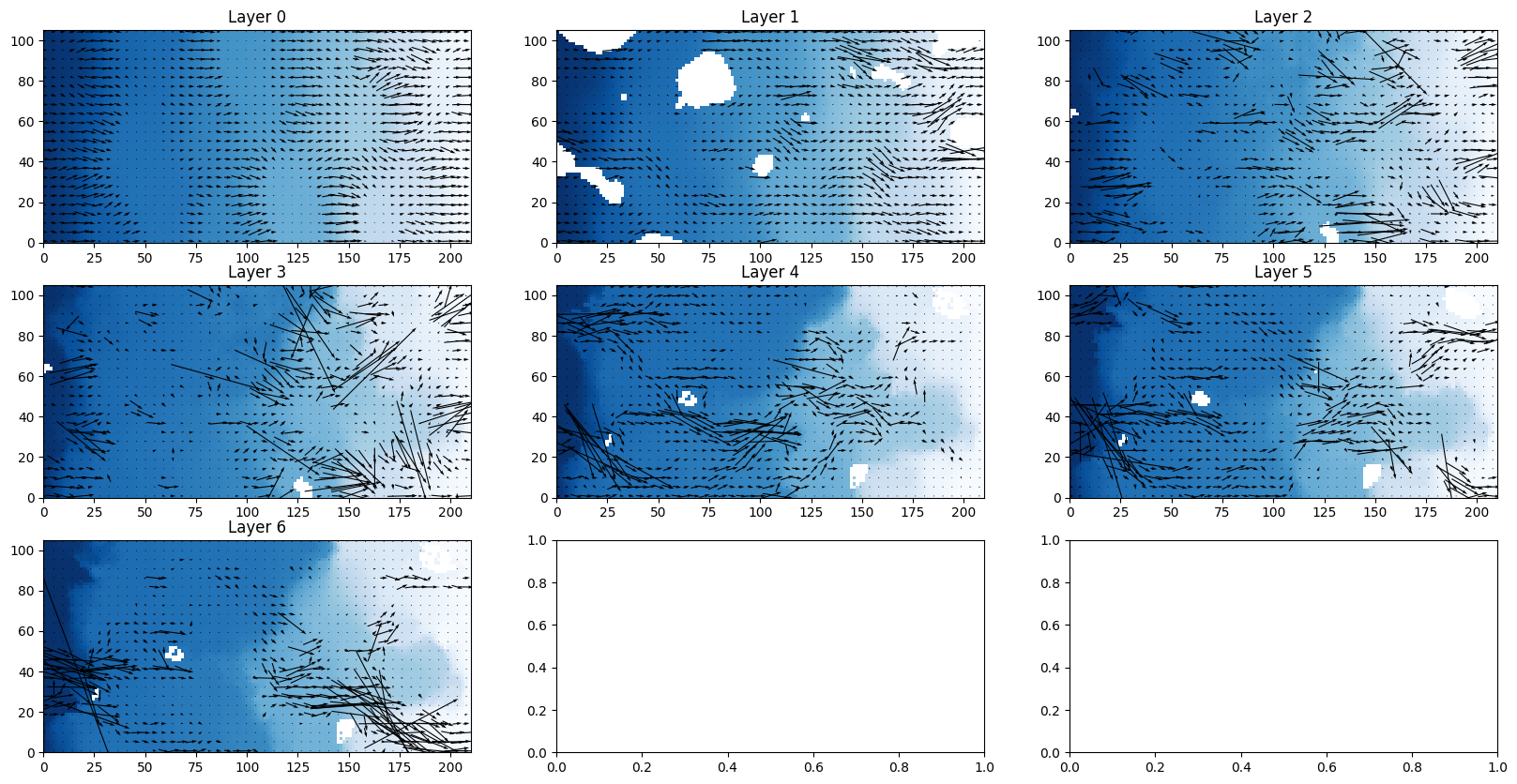
[47]:
# plots
fig, ax = plt.subplots(3, 3, figsize=(20, 10))
axes = ax.flatten()
from flopy.plot import PlotMapView
for ilayer in range(gwf.modelgrid.nlay-1):
    mapview = PlotMapView(model=gwf, layer=ilayer, ax=axes[ilayer])
    quadmesh = mapview.plot_array(heads[ilayer], cmap="Blues")
    mapview.plot_vector(qx[ilayer], qy[ilayer], color="black", istep=3, jstep=3)
    axes[ilayer].set_title("Layer {}".format(ilayer))
[48]:
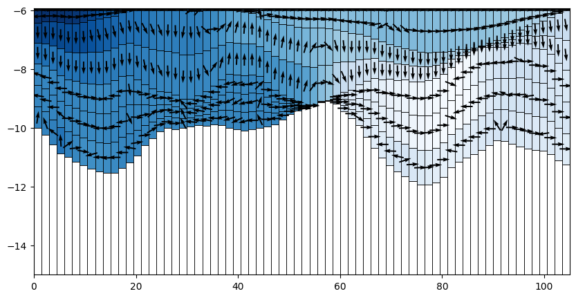
# plot cross section
from flopy.plot import PlotCrossSection
fig, ax = plt.subplots(1, 1, figsize=(10, 5))
cross_section = PlotCrossSection(model=gwf, line={"column": 40})
cross_section.plot_array(heads, cmap="Blues", ax=ax)
cross_section.plot_vector(qx, qy, qz, color="black", normalize=True)
cross_section.plot_grid(linewidth=0.5, color="black")
[48]:
<matplotlib.collections.PatchCollection at 0x1f0a92e6cd0>
[49]:
# flow pathlines
archpy_flow.prt_create(prt_name="test_prt", workspace="ws_prt", trackdir="backward",
                      list_p_coords=[(170.7, 99.75, -7), (170.7, 99.75, -9)])
C:\Users\schorppl\.conda\envs\archpy\Lib\site-packages\flopy\utils\gridintersect.py:290: DeprecationWarning: In the future this function will return a GeoDataFrame by default. Set geo_dataframe=True to adopt future behavior and silence this warning. Set geo_dataframe=False to silence this warning and maintain old behavior
  warnings.warn(
C:\Users\schorppl\.conda\envs\archpy\Lib\site-packages\flopy\utils\gridintersect.py:290: DeprecationWarning: In the future this function will return a GeoDataFrame by default. Set geo_dataframe=True to adopt future behavior and silence this warning. Set geo_dataframe=False to silence this warning and maintain old behavior
  warnings.warn(
[50]:
archpy_flow.prt_run(silent=False)
writing simulation...
  writing simulation name file...
  writing simulation tdis package...
  writing solution package ems...
  writing model test_prt...
    writing model name file...
    writing package mip...
    writing package dis...
    writing package prp...
    writing package oc...
    writing package fmi...
FloPy is using the following executable to run the model: \\home\schorppl$\exe\mf6.exe
                                   MODFLOW 6
                U.S. GEOLOGICAL SURVEY MODULAR HYDROLOGIC MODEL
                            VERSION 6.7.0 02/05/2026

   MODFLOW 6 compiled Feb 05 2026 22:36:44 with Intel(R) Fortran Intel(R) 64
   Compiler Classic for applications running on Intel(R) 64, Version 2021.6.0
                             Build 20220226_000000

This software has been approved for release by the U.S. Geological
Survey (USGS). Although the software has been subjected to rigorous
review, the USGS reserves the right to update the software as needed
pursuant to further analysis and review. No warranty, expressed or
implied, is made by the USGS or the U.S. Government as to the
functionality of the software and related material nor shall the
fact of release constitute any such warranty. Furthermore, the
software is released on condition that neither the USGS nor the U.S.
Government shall be held liable for any damages resulting from its
authorized or unauthorized use. Also refer to the USGS Water
Resources Software User Rights Notice for complete use, copyright,
and distribution information.


 MODFLOW runs in SEQUENTIAL mode

 Run start date and time (yyyy/mm/dd hh:mm:ss): 2026/04/01 10:39:31

 Writing simulation list file: mfsim.lst
 Using Simulation name file: mfsim.nam

    Solving:  Stress period:     1    Time step:     1

 Run end date and time (yyyy/mm/dd hh:mm:ss): 2026/04/01 10:39:32
 Elapsed run time:  0.260 Seconds

 Normal termination of simulation.
[51]:
path = archpy_flow.prt_get_pathlines(i_particle=2)
[52]:
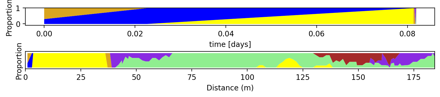
df_pi = archpy_flow.prt_get_facies_path_particle(2, fac_time=1/86400)
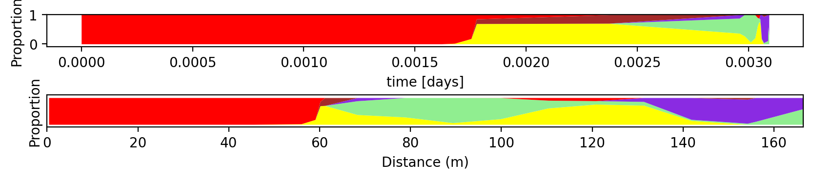
As cells were averages into layers, facies too and facies sequences encountered by particles are proportions of facies
[53]:
ArchPy.ap_mf.plot_particle_facies_sequence(T1, df=df_pi, plot_distance=True, proportions=True, plot_time=True)
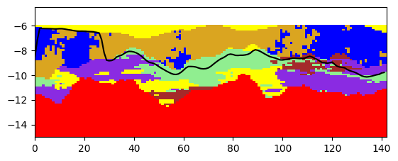
we can plot the particle course in the original archpy model to check if proportions are correct
[54]:
facies_smpl = []
facies = T1.get_facies()
for ix, iy in zip(*df_pi[["x", "y"]].T.values):
    idx_y, idx_x = T1.coord2cell(x= ix, y=iy)
    facies_smpl.append(facies[0, 0, :, idx_y, idx_x])
arr_facies = np.array(facies_smpl).T
arr_plot = np.ones([*arr_facies.shape, 4])

for iv in np.unique(arr_facies):

    if iv != 0:
        arr_plot[arr_facies == iv, :] = matplotlib.colors.to_rgba(T1.get_facies_obj(ID = iv, type="ID").c)
    else:
        arr_plot[arr_facies == iv, :] = (1, 1, 1, 1)
plt.imshow(arr_plot, origin="lower", interpolation="none", extent=[0, df_pi.shape[0], T1.oz, T1.oz + T1.nz*T1.sz], aspect=5)
plt.plot(df_pi["z"], c="k")
[54]:
[<matplotlib.lines.Line2D at 0x1f0a8ea4c10>]
[55]:
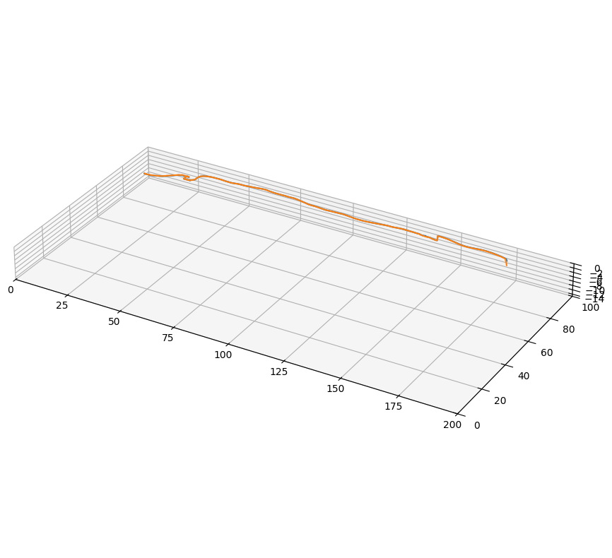
# 3D plot of the pathlines
fig = plt.figure(figsize=(10, 10))
ax = fig.add_subplot(111, projection="3d")

for i in range(3):
    path = archpy_flow.prt_get_pathlines(i_particle=i+1)
    plt.plot(path["x"], path["y"], path["z"])

plt.xlim(0, 200)
plt.ylim(0, 100)
ax.set_zlim(-15, 0)
ax.set_aspect("equal")
plt.show()
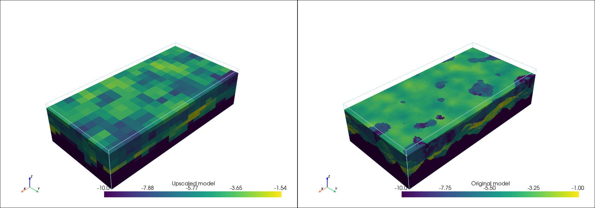
Upscaled model
Let us see now the upscaled model. Here we use the new_resolution mode. We upscale the model by a factor of 4 in x direction and 2 in y and z directions.
[56]:
T1.nx
[56]:
140
[57]:
archpy_flow = archpy2modflow(T1, exe_name="../../../../exe/mf6.exe")
archpy_flow.create_sim(grid_mode="new_resolution", iu=0, factor_x=7, factor_y=7, factor_z=7)
archpy_flow.set_k(k_key="K", iu=0, ifa=0, ip=0, log=True,
                k_average_method="new_resolution", average_facies=True)
Simulation created with the following parameters:
Grid mode: new_resolution
To retrieve the simulation, use the get_sim() method
[58]:
sim = archpy_flow.get_sim()
gwf = archpy_flow.get_gwf()
[59]:
pv.set_jupyter_backend("static")
[60]:
pl = pv.Plotter(shape=(1, 2), window_size=[2000, 700])
v_ex=5
sim = archpy_flow.get_sim()
gwf = archpy_flow.get_gwf()
arr = np.log10(gwf.npf.k33.array)
arr[arr==arr[0, 0, 0]] = np.nan
arr = np.flip(np.flipud(arr), axis=1)
im = geone.img.Img(nx=arr.shape[2], ny=arr.shape[1], nz=arr.shape[0], sx=gwf.dis.delr[0], sy=gwf.dis.delc[0], sz=1.05*v_ex, val=arr, nv=1,
                   varname=["Upscaled model"])
geone.imgplot3d.drawImage3D_surface(im, plotter=pl)

pl.subplot(0, 1)
arr = T1.get_prop("K", 0, 0, 0, all_data=False)
im = geone.img.Img(nx=arr.shape[2], ny=arr.shape[1], nz=arr.shape[0], sx=1.5, sy=1.5, sz=0.15*v_ex, nv=1,
                    val=arr.reshape(1, *arr.shape), varname=["Original model"])
geone.imgplot3d.drawImage3D_surface(im, plotter=pl)

pl.show()
[61]:
# add BC at left and right on all layers
h1 = 10
h2 = 0
chd_data = []

a = np.zeros((gwf.modelgrid.nlay, gwf.modelgrid.nrow, gwf.modelgrid.ncol), dtype=bool)
a[:, :, 0] = 1
lst_chd = array2cellids(a, gwf.dis.idomain.array)
for cellid in lst_chd:
    chd_data.append((cellid, h1))

a = np.zeros((gwf.modelgrid.nlay, gwf.modelgrid.nrow, gwf.modelgrid.ncol), dtype=bool)
a[:, :, -1] = 1
lst_chd = array2cellids(a, gwf.dis.idomain.array)
for cellid in lst_chd:
    chd_data.append((cellid, h2))

chd = fp.mf6.ModflowGwfchd(gwf, stress_period_data=chd_data, save_flows=True)
[62]:
sim.write_simulation()
sim.ims.complexity = "moderate"
sim.ims.write()
sim.run_simulation()
writing simulation...
  writing simulation name file...
  writing simulation tdis package...
  writing solution package ims_-1...
  writing model test...
    writing model name file...
    writing package dis...
    writing package ic...
    writing package oc...
    writing package npf...
    writing package chd_0...
INFORMATION: maxbound in ('', 'chd', 'dimensions') changed to 180 based on size of stress_period_data
FloPy is using the following executable to run the model: \\home\schorppl$\exe\mf6.exe
                                   MODFLOW 6
                U.S. GEOLOGICAL SURVEY MODULAR HYDROLOGIC MODEL
                            VERSION 6.7.0 02/05/2026

   MODFLOW 6 compiled Feb 05 2026 22:36:44 with Intel(R) Fortran Intel(R) 64
   Compiler Classic for applications running on Intel(R) 64, Version 2021.6.0
                             Build 20220226_000000

This software has been approved for release by the U.S. Geological
Survey (USGS). Although the software has been subjected to rigorous
review, the USGS reserves the right to update the software as needed
pursuant to further analysis and review. No warranty, expressed or
implied, is made by the USGS or the U.S. Government as to the
functionality of the software and related material nor shall the
fact of release constitute any such warranty. Furthermore, the
software is released on condition that neither the USGS nor the U.S.
Government shall be held liable for any damages resulting from its
authorized or unauthorized use. Also refer to the USGS Water
Resources Software User Rights Notice for complete use, copyright,
and distribution information.


 MODFLOW runs in SEQUENTIAL mode

 Run start date and time (yyyy/mm/dd hh:mm:ss): 2026/04/01 10:39:36

 Writing simulation list file: mfsim.lst
 Using Simulation name file: mfsim.nam

    Solving:  Stress period:     1    Time step:     1

 Run end date and time (yyyy/mm/dd hh:mm:ss): 2026/04/01 10:39:36
 Elapsed run time:  0.114 Seconds

 Normal termination of simulation.
[62]:
(True, [])
[63]:
mpexe_path = "../../../../exe/mp7.exe"
archpy_flow.prt_create(trackdir="backward",
                      list_p_coords=[(170.7, 99.75, -7), (170.7, 99.75, -9)])
archpy_flow.prt_run(silent=False)
C:\Users\schorppl\.conda\envs\archpy\Lib\site-packages\flopy\utils\gridintersect.py:290: DeprecationWarning: In the future this function will return a GeoDataFrame by default. Set geo_dataframe=True to adopt future behavior and silence this warning. Set geo_dataframe=False to silence this warning and maintain old behavior
  warnings.warn(
writing simulation...
  writing simulation name file...
  writing simulation tdis package...
  writing solution package ems...
  writing model test...
    writing model name file...
    writing package mip...
    writing package dis...
    writing package prp...
    writing package oc...
    writing package fmi...
FloPy is using the following executable to run the model: \\home\schorppl$\exe\mf6.exe
                                   MODFLOW 6
                U.S. GEOLOGICAL SURVEY MODULAR HYDROLOGIC MODEL
                            VERSION 6.7.0 02/05/2026

   MODFLOW 6 compiled Feb 05 2026 22:36:44 with Intel(R) Fortran Intel(R) 64
   Compiler Classic for applications running on Intel(R) 64, Version 2021.6.0
                             Build 20220226_000000

This software has been approved for release by the U.S. Geological
Survey (USGS). Although the software has been subjected to rigorous
review, the USGS reserves the right to update the software as needed
pursuant to further analysis and review. No warranty, expressed or
implied, is made by the USGS or the U.S. Government as to the
functionality of the software and related material nor shall the
fact of release constitute any such warranty. Furthermore, the
software is released on condition that neither the USGS nor the U.S.
Government shall be held liable for any damages resulting from its
authorized or unauthorized use. Also refer to the USGS Water
Resources Software User Rights Notice for complete use, copyright,
and distribution information.


 MODFLOW runs in SEQUENTIAL mode

 Run start date and time (yyyy/mm/dd hh:mm:ss): 2026/04/01 10:39:37

 Writing simulation list file: mfsim.lst
 Using Simulation name file: mfsim.nam

    Solving:  Stress period:     1    Time step:     1

 Run end date and time (yyyy/mm/dd hh:mm:ss): 2026/04/01 10:39:37
 Elapsed run time:  0.112 Seconds

 Normal termination of simulation.
[64]:
df_pi = archpy_flow.prt_get_facies_path_particle(1, fac_time=1/86400)
[65]:
ArchPy.ap_mf.plot_particle_facies_sequence(T1, df=df_pi, plot_distance=True, proportions=True, plot_time=True)
[66]:
path = archpy_flow.prt_get_pathlines()
fig = plt.figure(figsize=(10, 10))
ax = fig.add_subplot(111, projection="3d")

for ipth in range(1, 4):
    pth = path.loc[path.irpt==ipth]
    ax.plot(pth["x"], pth["y"], pth["z"])

plt.xlim(0, 200)
plt.ylim(0, 100)
ax.set_zlim(-15, 0)
ax.set_aspect("equal")
plt.show()

Comparisons
[67]:
np.random.seed(1)
# compare pathlines between the 3 modes

n_loc = 10
particles_loc_x = np.random.uniform(100, T1.get_xg()[-1], n_loc)
particles_loc_y = np.random.uniform(0, T1.get_yg()[-1], n_loc)
particles_loc_z = np.random.uniform(-12, -7, n_loc)
particles_loc = list(zip(particles_loc_x, particles_loc_y, particles_loc_z))
particles_loc.append((170.7, 99.75, -9))
n_loc += 1
[68]:
def add_chd(archpy_flow, h1=100, h2=0):

    # add BC at left and right on all layers
    chd_data = []

    gwf = archpy_flow.get_gwf()

    a = np.zeros((gwf.modelgrid.nlay, gwf.modelgrid.nrow, gwf.modelgrid.ncol), dtype=bool)
    a[:, :, 0] = 1
    lst_chd = array2cellids(a, gwf.dis.idomain.array)
    for cellid in lst_chd:
        chd_data.append((cellid, h1))

    a = np.zeros((gwf.modelgrid.nlay, gwf.modelgrid.nrow, gwf.modelgrid.ncol), dtype=bool)
    a[:, :, -1] = 1
    lst_chd = array2cellids(a, gwf.dis.idomain.array)
    for cellid in lst_chd:
        chd_data.append((cellid, h2))

    chd = fp.mf6.ModflowGwfchd(gwf, stress_period_data=chd_data, save_flows=True)
[69]:
iu = 0
ifa = 0

modflow_path = "../../../../exe/mf6.exe"

# Archpy grid mode #
archpy_flow = archpy2modflow(T1, exe_name=modflow_path)
archpy_flow.create_sim(grid_mode="archpy", iu=iu)
archpy_flow.set_k("K", iu, ifa, 0, log=True, average_facies=True)

sim = archpy_flow.get_sim()
gwf = archpy_flow.get_gwf()

add_chd(archpy_flow, 10, 0)

# modify ims to a more strict convergence criteria
sim.ims.remove()
inner_dvclose = 1e-4
ims = fp.mf6.ModflowIms(sim, complexity="moderate", inner_dvclose=inner_dvclose)

# set IC to help the model converge
dis = gwf.get_package("DIS")
ny, nx, nz = dis.nrow.get_data(), dis.ncol.get_data(), dis.nlay.get_data()
strt = np.linspace(10, 0, nx)
strt = np.tile(strt, (ny, 1))
strt = np.tile(strt, (nz, 1, 1))

archpy_flow.set_strt(strt)

sim.write_simulation()
sim.run_simulation()

archpy_flow.prt_create(
                      trackdir="backward",
                      list_p_coords=particles_loc)
archpy_flow.prt_run(silent=False)

l_df_pi = []
for pi in range(n_loc):
    df_pi = archpy_flow.prt_get_facies_path_particle(pi, fac_time=1/86400)
    l_df_pi.append(df_pi)

# Layers grid mode #
archpy_flow = archpy2modflow(T1, exe_name=modflow_path)
archpy_flow.create_sim(grid_mode="layers", iu=iu)
archpy_flow.set_k("K", iu, ifa, 0, log=True, average_facies=True)

sim = archpy_flow.get_sim()

add_chd(archpy_flow, 10, 0)

sim.write_simulation()
sim.ims.complexity = "moderate"
sim.ims.write()
sim.run_simulation()

archpy_flow.prt_create(
                        trackdir="backward",
                        list_p_coords=particles_loc)
archpy_flow.prt_run(silent=False)

l_df_pi_layers = []
for pi in range(n_loc):
    df_pi = archpy_flow.prt_get_facies_path_particle(pi, fac_time=1/86400)
    l_df_pi_layers.append(df_pi)

# New resolution grid mode #
archpy_flow = archpy2modflow(T1, exe_name=modflow_path)
archpy_flow.create_sim(grid_mode="new_resolution", iu=iu, factor_x=7, factor_y=7, factor_z=7)
archpy_flow.set_k("K", iu, ifa, 0, log=True, k_average_method="new_resolution", average_facies=True)

sim = archpy_flow.get_sim()

add_chd(archpy_flow, 10, 0)

sim.write_simulation()
sim.ims.complexity = "moderate"
sim.ims.write()
sim.run_simulation()

archpy_flow.prt_create(
                        trackdir="backward",
                        list_p_coords=particles_loc)
archpy_flow.prt_run(silent=False)

l_df_pi_new_res = []
for pi in range(n_loc):
    df_pi = archpy_flow.prt_get_facies_path_particle(pi, fac_time=1/86400)
    l_df_pi_new_res.append(df_pi)
Simulation created with the following parameters:
Grid mode: archpy
To retrieve the simulation, use the get_sim() method
writing simulation...
  writing simulation name file...
  writing simulation tdis package...
  writing solution package ims_-1...
  writing model test...
    writing model name file...
    writing package dis...
    writing package oc...
    writing package npf...
    writing package chd_0...
INFORMATION: maxbound in ('', 'chd', 'dimensions') changed to 8400 based on size of stress_period_data
    writing package ic...
FloPy is using the following executable to run the model: \\home\schorppl$\exe\mf6.exe
                                   MODFLOW 6
                U.S. GEOLOGICAL SURVEY MODULAR HYDROLOGIC MODEL
                            VERSION 6.7.0 02/05/2026

   MODFLOW 6 compiled Feb 05 2026 22:36:44 with Intel(R) Fortran Intel(R) 64
   Compiler Classic for applications running on Intel(R) 64, Version 2021.6.0
                             Build 20220226_000000

This software has been approved for release by the U.S. Geological
Survey (USGS). Although the software has been subjected to rigorous
review, the USGS reserves the right to update the software as needed
pursuant to further analysis and review. No warranty, expressed or
implied, is made by the USGS or the U.S. Government as to the
functionality of the software and related material nor shall the
fact of release constitute any such warranty. Furthermore, the
software is released on condition that neither the USGS nor the U.S.
Government shall be held liable for any damages resulting from its
authorized or unauthorized use. Also refer to the USGS Water
Resources Software User Rights Notice for complete use, copyright,
and distribution information.


 MODFLOW runs in SEQUENTIAL mode

 Run start date and time (yyyy/mm/dd hh:mm:ss): 2026/04/01 10:39:43

 Writing simulation list file: mfsim.lst
 Using Simulation name file: mfsim.nam

    Solving:  Stress period:     1    Time step:     1

 Run end date and time (yyyy/mm/dd hh:mm:ss): 2026/04/01 10:40:08
 Elapsed run time: 25.556 Seconds

 Normal termination of simulation.
C:\Users\schorppl\.conda\envs\archpy\Lib\site-packages\flopy\utils\gridintersect.py:290: DeprecationWarning: In the future this function will return a GeoDataFrame by default. Set geo_dataframe=True to adopt future behavior and silence this warning. Set geo_dataframe=False to silence this warning and maintain old behavior
  warnings.warn(
writing simulation...
  writing simulation name file...
  writing simulation tdis package...
  writing solution package ems...
  writing model test...
    writing model name file...
    writing package mip...
    writing package dis...
    writing package prp...
    writing package oc...
    writing package fmi...
FloPy is using the following executable to run the model: \\home\schorppl$\exe\mf6.exe
                                   MODFLOW 6
                U.S. GEOLOGICAL SURVEY MODULAR HYDROLOGIC MODEL
                            VERSION 6.7.0 02/05/2026

   MODFLOW 6 compiled Feb 05 2026 22:36:44 with Intel(R) Fortran Intel(R) 64
   Compiler Classic for applications running on Intel(R) 64, Version 2021.6.0
                             Build 20220226_000000

This software has been approved for release by the U.S. Geological
Survey (USGS). Although the software has been subjected to rigorous
review, the USGS reserves the right to update the software as needed
pursuant to further analysis and review. No warranty, expressed or
implied, is made by the USGS or the U.S. Government as to the
functionality of the software and related material nor shall the
fact of release constitute any such warranty. Furthermore, the
software is released on condition that neither the USGS nor the U.S.
Government shall be held liable for any damages resulting from its
authorized or unauthorized use. Also refer to the USGS Water
Resources Software User Rights Notice for complete use, copyright,
and distribution information.


 MODFLOW runs in SEQUENTIAL mode

 Run start date and time (yyyy/mm/dd hh:mm:ss): 2026/04/01 10:40:12

 Writing simulation list file: mfsim.lst
 Using Simulation name file: mfsim.nam

    Solving:  Stress period:     1    Time step:     1

 Run end date and time (yyyy/mm/dd hh:mm:ss): 2026/04/01 10:40:14
 Elapsed run time:  1.491 Seconds

 Normal termination of simulation.
No particle found
Simulation created with the following parameters:
Grid mode: layers
To retrieve the simulation, use the get_sim() method
writing simulation...
  writing simulation name file...
  writing simulation tdis package...
  writing solution package ims_-1...
  writing model test...
    writing model name file...
    writing package dis...
    writing package ic...
    writing package oc...
    writing package npf...
    writing package chd_0...
INFORMATION: maxbound in ('', 'chd', 'dimensions') changed to 536 based on size of stress_period_data
FloPy is using the following executable to run the model: \\home\schorppl$\exe\mf6.exe
                                   MODFLOW 6
                U.S. GEOLOGICAL SURVEY MODULAR HYDROLOGIC MODEL
                            VERSION 6.7.0 02/05/2026

   MODFLOW 6 compiled Feb 05 2026 22:36:44 with Intel(R) Fortran Intel(R) 64
   Compiler Classic for applications running on Intel(R) 64, Version 2021.6.0
                             Build 20220226_000000

This software has been approved for release by the U.S. Geological
Survey (USGS). Although the software has been subjected to rigorous
review, the USGS reserves the right to update the software as needed
pursuant to further analysis and review. No warranty, expressed or
implied, is made by the USGS or the U.S. Government as to the
functionality of the software and related material nor shall the
fact of release constitute any such warranty. Furthermore, the
software is released on condition that neither the USGS nor the U.S.
Government shall be held liable for any damages resulting from its
authorized or unauthorized use. Also refer to the USGS Water
Resources Software User Rights Notice for complete use, copyright,
and distribution information.


 MODFLOW runs in SEQUENTIAL mode

 Run start date and time (yyyy/mm/dd hh:mm:ss): 2026/04/01 10:40:15

 Writing simulation list file: mfsim.lst
 Using Simulation name file: mfsim.nam

    Solving:  Stress period:     1    Time step:     1

 Run end date and time (yyyy/mm/dd hh:mm:ss): 2026/04/01 10:40:16
 Elapsed run time:  0.467 Seconds

 Normal termination of simulation.
writing simulation...
  writing simulation name file...
  writing simulation tdis package...
  writing solution package ems...
  writing model test...
    writing model name file...
    writing package mip...
C:\Users\schorppl\.conda\envs\archpy\Lib\site-packages\flopy\utils\gridintersect.py:290: DeprecationWarning: In the future this function will return a GeoDataFrame by default. Set geo_dataframe=True to adopt future behavior and silence this warning. Set geo_dataframe=False to silence this warning and maintain old behavior
  warnings.warn(
    writing package dis...
    writing package prp...
    writing package oc...
    writing package fmi...
FloPy is using the following executable to run the model: \\home\schorppl$\exe\mf6.exe
                                   MODFLOW 6
                U.S. GEOLOGICAL SURVEY MODULAR HYDROLOGIC MODEL
                            VERSION 6.7.0 02/05/2026

   MODFLOW 6 compiled Feb 05 2026 22:36:44 with Intel(R) Fortran Intel(R) 64
   Compiler Classic for applications running on Intel(R) 64, Version 2021.6.0
                             Build 20220226_000000

This software has been approved for release by the U.S. Geological
Survey (USGS). Although the software has been subjected to rigorous
review, the USGS reserves the right to update the software as needed
pursuant to further analysis and review. No warranty, expressed or
implied, is made by the USGS or the U.S. Government as to the
functionality of the software and related material nor shall the
fact of release constitute any such warranty. Furthermore, the
software is released on condition that neither the USGS nor the U.S.
Government shall be held liable for any damages resulting from its
authorized or unauthorized use. Also refer to the USGS Water
Resources Software User Rights Notice for complete use, copyright,
and distribution information.


 MODFLOW runs in SEQUENTIAL mode

 Run start date and time (yyyy/mm/dd hh:mm:ss): 2026/04/01 10:40:16

 Writing simulation list file: mfsim.lst
 Using Simulation name file: mfsim.nam

    Solving:  Stress period:     1    Time step:     1

 Run end date and time (yyyy/mm/dd hh:mm:ss): 2026/04/01 10:40:16
 Elapsed run time:  0.207 Seconds

 Normal termination of simulation.
No particle found
Simulation created with the following parameters:
Grid mode: new_resolution
To retrieve the simulation, use the get_sim() method
writing simulation...
  writing simulation name file...
  writing simulation tdis package...
  writing solution package ims_-1...
  writing model test...
    writing model name file...
    writing package dis...
    writing package ic...
    writing package oc...
    writing package npf...
    writing package chd_0...
INFORMATION: maxbound in ('', 'chd', 'dimensions') changed to 180 based on size of stress_period_data
FloPy is using the following executable to run the model: \\home\schorppl$\exe\mf6.exe
                                   MODFLOW 6
                U.S. GEOLOGICAL SURVEY MODULAR HYDROLOGIC MODEL
                            VERSION 6.7.0 02/05/2026

   MODFLOW 6 compiled Feb 05 2026 22:36:44 with Intel(R) Fortran Intel(R) 64
   Compiler Classic for applications running on Intel(R) 64, Version 2021.6.0
                             Build 20220226_000000

This software has been approved for release by the U.S. Geological
Survey (USGS). Although the software has been subjected to rigorous
review, the USGS reserves the right to update the software as needed
pursuant to further analysis and review. No warranty, expressed or
implied, is made by the USGS or the U.S. Government as to the
functionality of the software and related material nor shall the
fact of release constitute any such warranty. Furthermore, the
software is released on condition that neither the USGS nor the U.S.
Government shall be held liable for any damages resulting from its
authorized or unauthorized use. Also refer to the USGS Water
Resources Software User Rights Notice for complete use, copyright,
and distribution information.


 MODFLOW runs in SEQUENTIAL mode

 Run start date and time (yyyy/mm/dd hh:mm:ss): 2026/04/01 10:40:18

 Writing simulation list file: mfsim.lst
 Using Simulation name file: mfsim.nam

    Solving:  Stress period:     1    Time step:     1

 Run end date and time (yyyy/mm/dd hh:mm:ss): 2026/04/01 10:40:18
 Elapsed run time:  0.118 Seconds

 Normal termination of simulation.
writing simulation...
  writing simulation name file...
C:\Users\schorppl\.conda\envs\archpy\Lib\site-packages\flopy\utils\gridintersect.py:290: DeprecationWarning: In the future this function will return a GeoDataFrame by default. Set geo_dataframe=True to adopt future behavior and silence this warning. Set geo_dataframe=False to silence this warning and maintain old behavior
  warnings.warn(
  writing simulation tdis package...
  writing solution package ems...
  writing model test...
    writing model name file...
    writing package mip...
    writing package dis...
    writing package prp...
    writing package oc...
    writing package fmi...
FloPy is using the following executable to run the model: \\home\schorppl$\exe\mf6.exe
                                   MODFLOW 6
                U.S. GEOLOGICAL SURVEY MODULAR HYDROLOGIC MODEL
                            VERSION 6.7.0 02/05/2026

   MODFLOW 6 compiled Feb 05 2026 22:36:44 with Intel(R) Fortran Intel(R) 64
   Compiler Classic for applications running on Intel(R) 64, Version 2021.6.0
                             Build 20220226_000000

This software has been approved for release by the U.S. Geological
Survey (USGS). Although the software has been subjected to rigorous
review, the USGS reserves the right to update the software as needed
pursuant to further analysis and review. No warranty, expressed or
implied, is made by the USGS or the U.S. Government as to the
functionality of the software and related material nor shall the
fact of release constitute any such warranty. Furthermore, the
software is released on condition that neither the USGS nor the U.S.
Government shall be held liable for any damages resulting from its
authorized or unauthorized use. Also refer to the USGS Water
Resources Software User Rights Notice for complete use, copyright,
and distribution information.


 MODFLOW runs in SEQUENTIAL mode

 Run start date and time (yyyy/mm/dd hh:mm:ss): 2026/04/01 10:40:18

 Writing simulation list file: mfsim.lst
 Using Simulation name file: mfsim.nam

    Solving:  Stress period:     1    Time step:     1

 Run end date and time (yyyy/mm/dd hh:mm:ss): 2026/04/01 10:40:18
 Elapsed run time:  0.122 Seconds

 Normal termination of simulation.
No particle found
[70]:
ArchPy.ap_mf.plot_particle_facies_sequence(archpy_flow.T1, l_df_pi[8], plot_distance=True)

[71]:
fig = plt.figure(figsize=(10, 10))
ax = fig.add_subplot(111, projection="3d")

for df in l_df_pi:
    if df is not None:
        ax.plot(df["x"], df["y"], df["z"])

plt.xlim(0, 200)
plt.ylim(0, 100)
ax.set_zlim(-15, -5)
ax.set_aspect("equalxy")
plt.show()

Next cell allows to visually compare pathlines of a specific particle between the three modes.
[72]:
%matplotlib inline
fig = plt.figure(figsize=(10, 10))
ax = fig.add_subplot(111, projection="3d")

i_particle = 3
for df in [l_df_pi[i_particle]]:
    ax.plot(df["x"], df["y"], df["z"], color="k")

for df in [l_df_pi_layers[i_particle]]:
    ax.plot(df["x"], df["y"], df["z"], color="r")
    # ax.scatter(df["x"], df["y"], df["z"], color="r")
for df in [l_df_pi_new_res[i_particle]]:
    ax.plot(df["x"], df["y"], df["z"], color="b")

plt.xlim(0, 200)
plt.ylim(0, 100)
ax.set_zlim(-15, -5)
ax.set_aspect("equalxy")
plt.show()
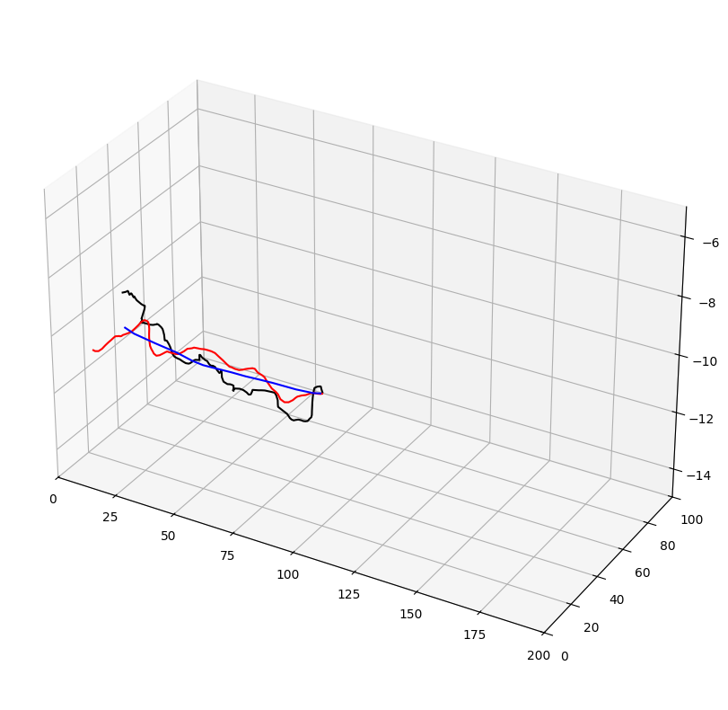
However, this is not sufficient to exactly determine the impact of upscaling on pathlines, we need to quantify the differences between the curves.
The following cell shows a comparison between the three modes. The pathlines are compared using different distance (Frechet, Hausdorff, and DTW)
[73]:
# write a function to compute the frechet distance between two pathlines
import scipy
from scipy.spatial import distance

def DTW(path1, path2):
    """
    Compute the Dynamic Time Warping distance between two pathlines (path1 and path2)
    """

    # compute the distance between each point of the two pathlines
    dist = distance.cdist(path1, path2)

    # compute frechet matrix
    MF = np.zeros(dist.shape)
    for i in range(dist.shape[0]):
        for j in range(dist.shape[1]):
            if i == 0 and j == 0:
                MF[i, j] = dist[i, j]
            elif i == 0:
                MF[i, j] = dist[i, j]
            elif j == 0:
                MF[i, j] = dist[i, j]
            else:
                MF[i, j] = dist[i, j] + min(MF[i-1, j], MF[i, j-1], MF[i-1, j-1])

    return MF[-1, -1]

def frechet_distance(path1, path2):

    """
    Compute the Frechet distance between two pathlines (2D array of shape (n_points, 3))

    """

    # compute the distance between each point of the two pathlines
    dist = distance.cdist(path1, path2)

    # compute frechet matrix
    MF = np.zeros(dist.shape)
    for i in range(dist.shape[0]):
        for j in range(dist.shape[1]):
            if i == 0 and j == 0:
                MF[i, j] = dist[i, j]
            elif i == 0:
                MF[i, j] = max(MF[i, j-1], dist[i, j])
            elif j == 0:
                MF[i, j] = max(MF[i-1, j], dist[i, j])
            else:
                MF[i, j] = max(min(MF[i-1, j], MF[i, j-1], MF[i-1, j-1]), dist[i, j])

    return MF[-1, -1]

def hausdorff_distance(path1, path2):
    """
    Compute the Hausdorff distance between two pathlines
    """

    from scipy.spatial.distance import directed_hausdorff

    d1 = directed_hausdorff(path1, path2)
    return d1[0]


l_layer_frechet = []
l_new_res_frechet = []
l_layer_hausdorff = []
l_new_res_hausdorff = []
l_layer_dtw = []
l_new_res_dtw = []
for i_particle in range(1, n_loc):
    if i_particle in []:
        pass
    else:
        # compute frechet and hausdorffdistance
        path1 = l_df_pi[i_particle][["x", "y", "z"]].values
        path2 = l_df_pi_layers[i_particle][["x", "y", "z"]].values
        l_layer_frechet.append(frechet_distance(path1, path2))
        l_layer_hausdorff.append(hausdorff_distance(path1, path2))

        path2 = l_df_pi_new_res[i_particle][["x", "y", "z"]].values
        l_new_res_frechet.append(frechet_distance(path1, path2))
        l_new_res_hausdorff.append(hausdorff_distance(path1, path2))

        # # DTW
        path1 = l_df_pi[i_particle][["x", "y", "z", "time"]]

        path2 = l_df_pi_layers[i_particle][["x", "y", "z", "time"]]

        # # merge the two dataframes on time
        df_merge = pd.merge(path1, path2, on="time", suffixes=("_1", "_2"), how="outer").fillna(method="ffill").set_index("time")
        path1 = df_merge[["x_1", "y_1", "z_1"]]
        path2 = df_merge[["x_2", "y_2", "z_2"]]

        l_layer_dtw.append(DTW(path1.values, path2.values))

        path1 = l_df_pi[i_particle][["x", "y", "z", "time"]]

        path2 = l_df_pi_new_res[i_particle][["x", "y", "z", "time"]]

        # # merge the two dataframes on time
        df_merge = pd.merge(path1, path2, on="time", suffixes=("_1", "_2"), how="outer").fillna(method="ffill").set_index("time")
        path1 = df_merge[["x_1", "y_1", "z_1"]]
        path2 = df_merge[["x_2", "y_2", "z_2"]]
        l_new_res_dtw.append(DTW(path1.values, path2.values))


fig, ax = plt.subplots(3, 1, figsize=(10, 8))
ax[0].plot(l_layer_frechet, label="Layers mode")
ax[0].plot(l_new_res_frechet, label="New resolution mode")
ax[0].set_xlabel("Particle")
ax[0].set_ylabel("Frechet distance")
ax[0].legend()

ax[1].plot(l_layer_hausdorff, label="Layers mode")
ax[1].plot(l_new_res_hausdorff, label="New resolution mode")
ax[1].set_xlabel("Particle")
ax[1].set_ylabel("Hausdorff distance")
ax[1].legend()

ax[2].plot(l_layer_dtw, label="Layers mode")
ax[2].plot(l_new_res_dtw, label="New resolution mode")
ax[2].set_xlabel("Particle")
ax[2].set_ylabel("DTW distance")
ax[2].legend()

plt.show()

print("Frechet distance")
print("Layers mode: ", np.mean(l_layer_frechet))
print("New resolution mode: ", np.mean(l_new_res_frechet))
print("Hausdorff distance")
print("Layers mode: ", np.mean(l_layer_hausdorff))
print("New resolution mode: ", np.mean(l_new_res_hausdorff))
print("DTW distance")
print("Layers mode: ", np.mean(l_layer_dtw))
print("New resolution mode: ", np.mean(l_new_res_dtw))
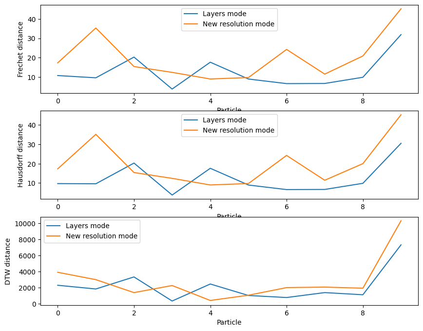
Frechet distance
Layers mode:  12.626855038079473
New resolution mode:  20.119001596763518
Hausdorff distance
Layers mode:  12.370150778497644
New resolution mode:  20.006027618993834
DTW distance
Layers mode:  2202.3531569456522
New resolution mode:  2850.0876545331253
This concludes this notebook on the basics of archpy2modflow.