3D model example
This notebook presents a full 3D model, purely synthetical, using various capabilities of ArchPy such as Truncated plurigaussian for filling and physical properties conditioning.
[1]:
import numpy as np
import matplotlib
from matplotlib import colors
import matplotlib.pyplot as plt
import geone
import geone.covModel as gcm
import geone.imgplot3d as imgplt3
import pyvista as pv
pv.set_jupyter_backend('static')
import sys

#For loading ArchPy, the path where ArchPy is must be added with sys
sys.path.append("../../")
#my modules
from ArchPy.base import * #ArchPy main functions
from ArchPy.tpgs import * #Truncated plurigaussians
[2]:
PB = Pile(name = "PB",seed=1)
P1 = Pile(name="P1",seed=1)
[3]:
#grid
sx = 1.5
sy = 1.5
sz = .15
x1 = 20
y1 = 10
z1 = -6
x0 = 0
y0 = 0
z0 = -15
nx = 133
ny = 67
nz = 62


dimensions = (nx, ny, nz)
spacing = (sx, sy, sz)
origin = (x0, y0, z0)
[4]:
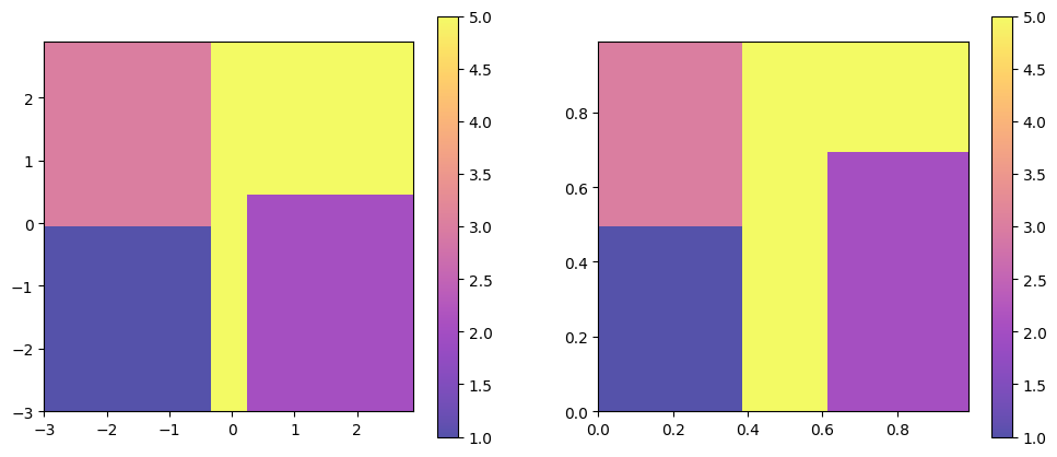
## setup TPGs for B units

#flag
#thresholds
t2g1 = -0.3
t3g1 = .3
t1g2 = 0
t2g2 = 0.5

#dictionnaries show where a certain facies is present.
# The structure is a list of list containing 2 tuples of size 2 that indicates the limits of the gaussian fields
# e.g. [[(lower_boundary1_g1,upper_boundary1_g1),(lower_boundary1_g2,upper_boundary1_g2)]] --> this indicates one cuboid and multiple can be defined
dic1 = [[(-np.inf,t2g1),(-np.inf,t1g2)]] # this facies is present between -inf to -0.3 of the 1st gaussian field and between -inf to 0 of the 2
dic2 = [[(t3g1,np.inf),(-np.inf,t2g2)]]
dic3 = [[(-np.inf,t2g1),(t1g2,np.inf)]]
dic4 = [[(t2g1,t3g1),(-np.inf,np.inf)],[(t3g1,np.inf),(t2g2,np.inf)]]

flag = {1:dic1,
        2:dic2,
        3:dic3,
        5:dic4}
print(ArchPy.tpgs.pfa(flag))


plt.figure(figsize=(12,5))
plt.subplot(1,2,1)
plot_flag(flag,alpha=.7)

plt.subplot(1,2,2)
plot_flag(Gspace2Pspace(flag),alpha=.7)

## G_cm
G1 = gcm.CovModel3D(elem=[("cubic",{"w":1.,"r":[50,50,20]}),
                         ("nugget",{"w":0.0})],name="G1")
G2 = gcm.CovModel3D(elem=[("cubic",{"w":1.,"r":[50,50,20]}),
                         ("nugget",{"w":0.0})],name="G2",alpha=30)
G_cm = [G1,G2]
[0.19104429 0.26419991 0.19104429 0.35371151]
[5]:
#units covmodel
covmodelD = gcm.CovModel2D(elem=[('cubic', {'w':0.6, 'r':[60,60]})])
covmodelC = gcm.CovModel2D(elem=[('cubic', {'w':0.2, 'r':[80,80]})])
covmodelB = gcm.CovModel2D(elem=[('cubic', {'w':0.6, 'r':[60,60]})])
covmodel_er = gcm.CovModel2D(elem=[('spherical', {'w':1, 'r':[100,100]})])

## facies covmodel
covmodel_SIS_C = gcm.CovModel3D(elem=[("exponential",{"w":.25,"r":[10,10,3]})],alpha=0,name="vario_SIS") # input variogram
covmodel_SIS_D = gcm.CovModel3D(elem=[("exponential",{"w":.25,"r":[5,5,5]})],alpha=0,name="vario_SIS") # input variogram
lst_covmodelC=[covmodel_SIS_C] # list of covmodels to pass at the function
lst_covmodelD=[covmodel_SIS_D]


#create Lithologies
dic_s_D = {"int_method" : "grf_ineq","covmodel" : covmodelD}
dic_f_D = {"f_method" : "TPGs","Flag" : flag,"G_cm":G_cm,"grf_method":"sgs"}
D = Unit(name="D",order=1,ID = 1,color="gold",contact="onlap",surface=Surface(contact="onlap",dic_surf=dic_s_D)
         ,dic_facies=dic_f_D)

dic_s_C = {"int_method" : "grf_ineq","covmodel" : covmodelC}
dic_f_C = {"f_method" : "SIS","neig" : 10,"f_covmodel":covmodel_SIS_C}
C = Unit(name="C",order=2,ID = 2,color="blue",contact="onlap",dic_facies=dic_f_C,surface=Surface(dic_surf=dic_s_C,contact="onlap"))

dic_s_er2 = {"int_method" : "grf","covmodel" : covmodel_er}
erosion2 = Surface(dic_surf=dic_s_er2, contact="erode")
#er2 = Unit(name="erosion2",ID = 4, order=4,contact="erode",color="black",surface=Surface(dic_surf = dic_s_er2,contact="erode"))

dic_s_B = {"int_method" : "grf_ineq","covmodel" : covmodelB}
dic_f_B = {"f_method":"SubPile","SubPile":PB}
B = Unit(name="B",order=3,ID = 3,color="green",contact="onlap",dic_facies=dic_f_B,surface=Surface(contact="onlap",dic_surf=dic_s_B))

dic_s_A = {"int_method":"grf_ineq","covmodel": covmodelB}
dic_f_A = {"f_method":"homogenous"}
A = Unit(name="A",order=5,ID = 5,color="red",contact="onlap",dic_facies=dic_f_A,surface=Surface(dic_surf = dic_s_A,contact="onlap"))

#Master pile
P1.add_unit([D,C,B,A])

# PB
ds_B3 = {"int_method":"grf_ineq","covmodel":covmodelB}
df_B3 = {"f_method":"SIS","neig" : 10,"f_covmodel":covmodel_SIS_D}
B3 = Unit(name = "B3",order=1,ID = 6,color="forestgreen",surface=Surface(dic_surf=ds_B3,contact="onlap"),dic_facies=df_B3)

ds_B2 = {"int_method":"grf_ineq","covmodel":covmodelB}
df_B2 = {"f_method":"SIS","neig" : 10,"f_covmodel":covmodel_SIS_D}
B2 = Unit(name = "B2",order=2,ID = 7,color="limegreen",surface=Surface(dic_surf=ds_B2,contact="erode"),dic_facies=df_B2)

ds_B1 = {"int_method":"grf_ineq","covmodel":covmodelB}
df_B1 = {"f_method":"SIS","neig" : 10,"f_covmodel":covmodel_SIS_D}
B1 = Unit(name = "B1",order=3, ID = 8,color="palegreen",surface=Surface(dic_surf=ds_B1,contact="onlap"),dic_facies=df_B1)

## Subpile
PB.add_unit([B3,B2,B1])
Unit D: Surface added for interpolation
Unit C: covmodel for SIS added
Unit C: Surface added for interpolation
Unit B: Surface added for interpolation
Unit A: Surface added for interpolation
Stratigraphic unit D added ✅
Stratigraphic unit C added ✅
Stratigraphic unit B added ✅
Stratigraphic unit A added ✅
Unit B3: covmodel for SIS added
Unit B3: Surface added for interpolation
Unit B2: covmodel for SIS added
Unit B2: Surface added for interpolation
Unit B1: covmodel for SIS added
Unit B1: Surface added for interpolation
Stratigraphic unit B3 added ✅
Stratigraphic unit B2 added ✅
Stratigraphic unit B1 added ✅
[6]:
# covmodels for the property model
covmodelK = gcm.CovModel3D(elem=[("exponential",{"w":0.3,"r":[5,5,1]})],alpha=-20,name="K_vario")
covmodelK2 = gcm.CovModel3D(elem=[("spherical",{"w":0.1,"r":[3,3,1]})],alpha=0,name="K_vario_2")
covmodelPoro = gcm.CovModel3D(elem=[("exponential",{"w":0.005,"r":[10,10,10]})],alpha=0,name="poro_vario")

facies_1 = Facies(ID = 1,name="Sand",color="yellow")
facies_2 = Facies(ID = 2,name="Gravel",color="lightgreen")
facies_3 = Facies(ID = 3,name="GM",color="blueviolet")
facies_4 = Facies(ID = 4,name="Clay",color="blue")
facies_5 = Facies(ID = 5,name="SM",color="brown")
facies_6 = Facies(ID = 6,name="Silt",color="goldenrod")
facies_7 = Facies(ID = 7,name="basement",color="red")

A.add_facies([facies_7])
B.add_facies([facies_1,facies_2,facies_3,facies_5])
D.add_facies([facies_1,facies_2,facies_3,facies_5])
C.add_facies([facies_4,facies_6])
#add same facies than B
for b in PB.list_units:
    b.add_facies(B.list_facies)

permea = Prop("K",[facies_1,facies_2,facies_3,facies_4,facies_5,facies_6,facies_7],
                  [covmodelK2,covmodelK,covmodelK,None,covmodelK2,covmodelK,None],
                  means=[-3.5,-2,-4.5,-8,-5.5,-6.5,-10],
                  int_method = ["sgs","sgs","sgs","homogenous","sgs","sgs","homogenous"],
                  def_mean=-5)
poro = Prop("Porosity",
            [facies_1,facies_3,facies_4],
            [covmodelPoro,covmodelPoro,covmodelPoro],
             means = [0.4,0.3,0.2],
             int_method = ["sgs","sgs","sgs"],
             def_mean=0.3,
             vmin=0)
Facies basement added to unit A ✅
Facies Sand added to unit B ✅
Facies Gravel added to unit B ✅
Facies GM added to unit B ✅
Facies SM added to unit B ✅
Facies Sand added to unit D ✅
Facies Gravel added to unit D ✅
Facies GM added to unit D ✅
Facies SM added to unit D ✅
Facies Clay added to unit C ✅
Facies Silt added to unit C ✅
Facies Sand added to unit B3 ✅
Facies Gravel added to unit B3 ✅
Facies GM added to unit B3 ✅
Facies SM added to unit B3 ✅
Facies Sand added to unit B2 ✅
Facies Gravel added to unit B2 ✅
Facies GM added to unit B2 ✅
Facies SM added to unit B2 ✅
Facies Sand added to unit B1 ✅
Facies Gravel added to unit B1 ✅
Facies GM added to unit B1 ✅
Facies SM added to unit B1 ✅
[7]:
top = np.ones([ny,nx])*-6
bot = np.ones([ny,nx])*z0
[8]:
#logs strati
log_strati1 = [(C,-6.01),(B3,-8),(B2,-9),(B1,-9.5),(A,-10)]
log_strati2 = [(C,-6.01),(B3,-8.5),(B2,-9.5),(A,-10.5)]
log_strati3 = [(D,-6.01),(B3,-8),(B2,-8.5),(B1,-9.5),(A,-10.5)]
log_strati4 = [(D,-6.01),(B3,-9),(B2,-10),(A,-11)]
log_strati5 = [(D,-6.01),(C,-10),(A,-12)]
log_strati6 = [(D,-6.01),(A,-9)]

# logs facies
log_facies1 = [(facies_4,-6.01),(facies_6,-6.5),(facies_4,-7),(facies_6,-7.5), # facies in unit C
               (facies_1,-8),(facies_5,-8.5),(facies_2,-9),(facies_3,-9.3),  # facies in unit B
               (facies_7,-10)]
log_facies2 = [(facies_4,-6.01),(facies_6,-7.3),(facies_4,-7.6),(facies_6,-8),
               (facies_2,-8.5),(facies_1,-8.8),(facies_2,-9),(facies_3,-9.2),(facies_1,-10),
               (facies_7,-10.5)]
log_facies3 = [(facies_1,-6.015),(facies_2,-6.8),(facies_5,-7),(facies_3,-7.3),(facies_1,-7.5),
               (facies_2,-8),(facies_1,-8.8),(facies_2,-9),(facies_3,-9.2),(facies_1,-10),
              (facies_7,-10.5)]
log_facies4 = [(facies_1,-6.01),(facies_2,-7.5),(facies_5,-7.8),(facies_3,-8),(facies_5,-8.3),(facies_1,-8.7),
               (facies_2,-9),(facies_1,-10),(facies_2,-10.5),
               (facies_7,-11)]
log_facies5 = [(facies_5,-6.01),(facies_1,-7.5),(facies_3,-7.8),(facies_2,-8),(facies_1,-8.3),(facies_2,-8.7),(facies_1,-9),(facies_5,-9.5),
               (facies_4,-10),(facies_6,-10.4),(facies_4,-11),
               (facies_7,-12)]
log_facies6 = [(facies_1,-6.01),(facies_2,-8.3),(facies_3,-8.5),(facies_2,-8.7),
               (facies_7,-9)]

#create boreholes
bh1 = borehole("b1", 1, x=10*1,y=10*5,z=log_strati1[0][1],depth =9,log_strati=log_strati1,log_facies=log_facies1)
bh2 = borehole("b2", "B", x=10*3,y=10*2,z=log_strati2[0][1],depth =8,log_strati=log_strati2,log_facies=log_facies2)
bh3 = borehole("b3", "C", x=10*5,y=10*6,z=log_strati3[0][1],depth =7,log_strati=log_strati3,log_facies=log_facies3)
bh4 = borehole("b4", "D", x=10*10,y=10*1,z=log_strati4[0][1],depth =8,log_strati=log_strati4,log_facies=log_facies4)
bh5 = borehole("b5", "E", x=10*15,y=10*3,z=log_strati5[0][1],depth =8,log_strati=log_strati5,log_facies=log_facies5)
bh6 = borehole("b6", "F", x=10*19,y=10*9,z=log_strati6[0][1],depth =6,log_strati=log_strati6,log_facies=log_facies6)
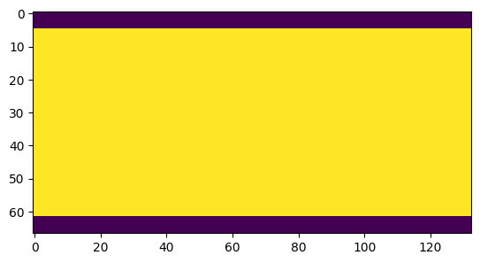
[9]:
domain = np.ones([ny,nx],dtype=bool)
domain[: 5]= 0
domain[-5:] = 0
plt.imshow(domain)
[9]:
<matplotlib.image.AxesImage at 0x1c9e6d87250>
[10]:
T1 = Arch_table(name = "P1",seed=1)
T1.set_Pile_master(P1)
T1.add_grid(dimensions, spacing, origin, top=top,bot=bot,polygon=domain)
T1.rem_all_bhs()
T1.add_bh([bh1,bh2,bh3,bh4,bh5,bh6])
T1.add_prop([permea])
Pile sets as Pile master
## Adding Grid ##
## Grid added and is now simulation grid ##
Standard boreholes removed
Fake boreholes removed
Geological map boreholes removed
Borehole 1 goes below model limits, borehole 1 depth cut
Borehole 1 added
Borehole B added
Borehole C added
Borehole D added
Borehole E added
Borehole F added
Property K added
[11]:
T1.process_bhs()
##### ORDERING UNITS #####
Pile P1: ordering units
Stratigraphic units have been sorted according to order
Discrepency in the orders for units A and B
Changing orders for that they range from 1 to n
Pile PB: ordering units
Stratigraphic units have been sorted according to order
hierarchical relations set
First altitude in log facies of bh C is not set at the top of the borehole, altitude changed

 ## Computing distributions for Normal Score Transform ##

Processing ended successfully
[12]:
# plot piles
T1.plot_pile()

[13]:
# display tables
T1.get_sp(unit_kws=["covmodel"])[0]
[13]:
| name | contact | int_method | covmodel | filling_method | list_facies | |
|---|---|---|---|---|---|---|
| 0 | D | onlap | grf_ineq | 0: cub (w: 0.6, r: [60, 60]) | TPGs | [Sand, Gravel, GM, SM] |
| 1 | C | onlap | grf_ineq | 0: cub (w: 0.2, r: [80, 80]) | SIS | [Clay, Silt] |
| 2 | B | onlap | grf_ineq | 0: cub (w: 0.6, r: [60, 60]) | SubPile | [Sand, Gravel, GM, SM] |
| 3 | A | onlap | grf_ineq | 0: cub (w: 0.6, r: [60, 60]) | homogenous | [basement] |
| 4 | B3 | onlap | grf_ineq | 0: cub (w: 0.6, r: [60, 60]) | SIS | [Sand, Gravel, GM, SM] |
| 5 | B2 | erode | grf_ineq | 0: cub (w: 0.6, r: [60, 60]) | SIS | [Sand, Gravel, GM, SM] |
| 6 | B1 | onlap | grf_ineq | 0: cub (w: 0.6, r: [60, 60]) | SIS | [Sand, Gravel, GM, SM] |
[14]:
T1.get_sp()[1]
[14]:
| name | property | mean | covmodels | |
|---|---|---|---|---|
| 0 | Sand | K | -3.500000 | 0: sph (w: 0.1, r: [3, 3, 1]) |
| 1 | Gravel | K | -2.000000 | 0: exp (w: 0.3, r: [5, 5, 1]) |
| 2 | GM | K | -4.500000 | 0: exp (w: 0.3, r: [5, 5, 1]) |
| 3 | SM | K | -5.500000 | 0: sph (w: 0.1, r: [3, 3, 1]) |
| 4 | Clay | K | -8.000000 | None |
| 5 | Silt | K | -6.500000 | 0: exp (w: 0.3, r: [5, 5, 1]) |
| 6 | basement | K | -10.000000 | None |
When you are computing the surface, you can decide to activate or not the vertical discretization (in case you are only interested in the simulated surfaces.) But beaware that you will not be able to proceed with facies and property modeling if you do so. by default it is set to true
[15]:
import ArchPy
[16]:
T1.ncpu = 8
[17]:
T1.verbose=0
[18]:
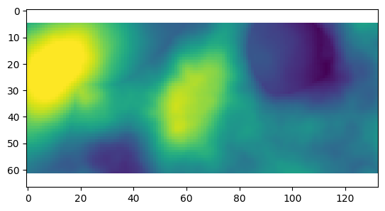
T1.compute_surf(1, vert_discret=True)
[19]:
plt.imshow(T1.get_surfaces_unit(C)[0])
[19]:
<matplotlib.image.AxesImage at 0x1c9e4b19790>
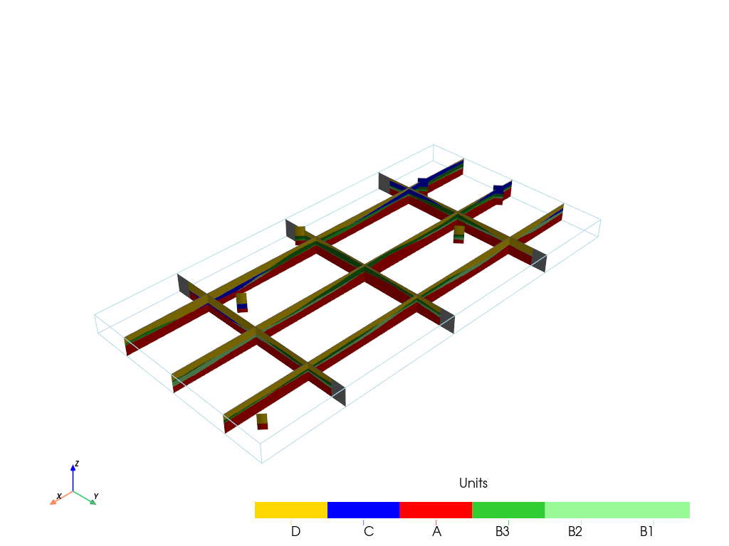
Plotting units
ArchPy integrates multiple plotting utilities that mostly rely on Pyvista and Geone. Below are some examples
[20]:
p = pv.Plotter()
v_ex = 1

T1.plot_units(0, v_ex=v_ex, plotter=p, slicex=(0.2, 0.5, 0.8), slicey=(0.2, 0.5, 0.8))
T1.plot_bhs(plotter=p, v_ex=v_ex)
p.show()
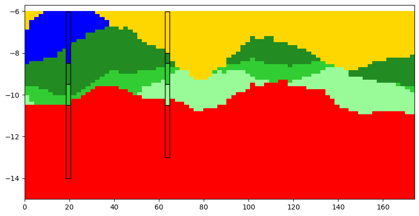
Cross-sections
ArchPy integrates the possibility to make cross-section, interactively or not. You can pass a list of point where to draw the cross-section. Boreholes are projected on the cross-section if they are at a distance less than dist_max. You can choose which realization to plot with iu parameter. The width of the boreholes can be set with width parameter.
[21]:
#cross section
#first a list of points must be defined
p1 = [10,10]
p2 = [50,70]
p3 = [150,90]
T1.plot_cross_section([p1,p2,p3],iu=0, ratio_aspect=2, dist_max=15, width=2, h_level=0, typ="units")
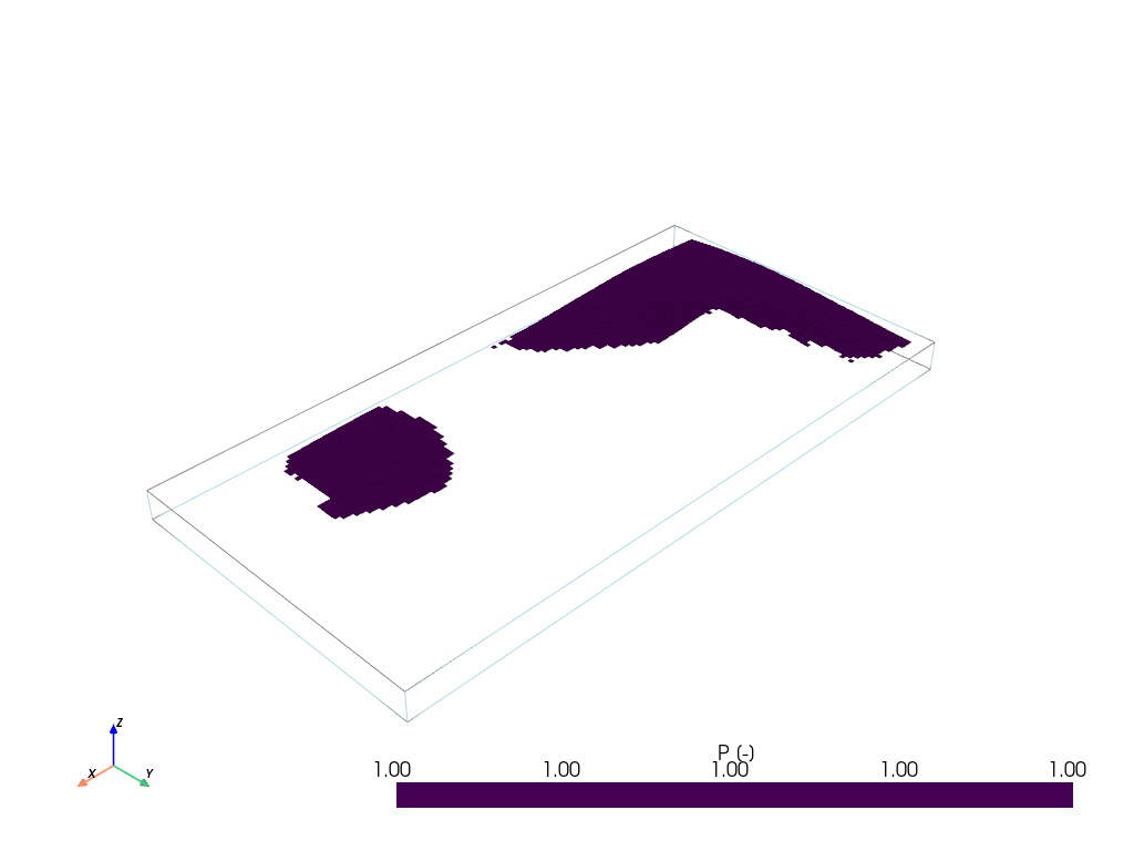
ArchPy also integrates probability plotting functions which allow to plot any ArchPy object such as units or facies
[22]:
T1.plot_proba(C, filtering_interval=[0.01, 1])
[23]:
T1.verbose=2
[24]:
T1.compute_facies(1, verbose_methods=3)
### Unit D: facies simulation with TPGs method ####
### Unit D - realization 0 ###
Time elapsed 2.58 s

### Unit C: facies simulation with SIS method ####
### Unit C - realization 0 ###
Only one facies covmodels for multiples facies, adapt sill to right proportions
simulateIndicator3D: Geos-Classic running... [VERSION 2.0 / BUILD NUMBER 20240322 / OpenMP 8 thread(s)]
simulateIndicator3D: Geos-Classic run complete
Time elapsed 0.06 s

### Unit B: facies simulation with SubPile method ####
SubPile filling method, nothing happened
Time elapsed 0.0 s

### Unit A: facies simulation with homogenous method ####
### Unit A - realization 0 ###
Time elapsed 0.0 s

### Unit B3: facies simulation with SIS method ####
### Unit B3 - realization 0 ###
Only one facies covmodels for multiples facies, adapt sill to right proportions
simulateIndicator3D: Geos-Classic running... [VERSION 2.0 / BUILD NUMBER 20240322 / OpenMP 8 thread(s)]
simulateIndicator3D: Geos-Classic run complete
Time elapsed 0.12 s

### Unit B2: facies simulation with SIS method ####
### Unit B2 - realization 0 ###
Only one facies covmodels for multiples facies, adapt sill to right proportions
simulateIndicator3D: Geos-Classic running... [VERSION 2.0 / BUILD NUMBER 20240322 / OpenMP 8 thread(s)]
simulateIndicator3D: Geos-Classic run complete
Time elapsed 0.06 s

### Unit B1: facies simulation with SIS method ####
### Unit B1 - realization 0 ###
Only one facies covmodels for multiples facies, adapt sill to right proportions
simulateIndicator3D: Geos-Classic running... [VERSION 2.0 / BUILD NUMBER 20240322 / OpenMP 8 thread(s)]
simulateIndicator3D: Geos-Classic run complete
Time elapsed 0.1 s

### 2.92: Total time elapsed for computing facies ###
[25]:
T1.plot_facies(v_ex=v_ex)

[26]:
T1.plot_facies(0,0,inside_units=[B], v_ex=v_ex)

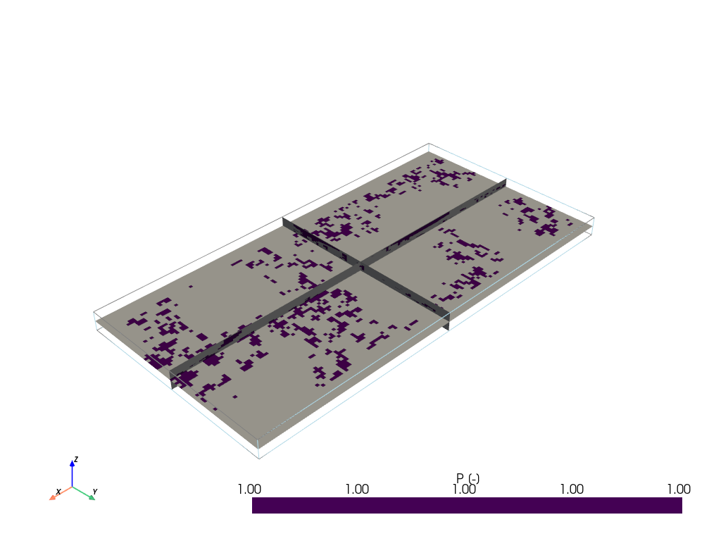
[27]:
T1.plot_proba(facies_1,filtering_interval=[0.1,1],slicex=0.5,slicey=0.5,slicez=0.5, v_ex=v_ex) # sand
Property hard data can be passed by a list of coordinates and values
[28]:
#prop hd

ix = np.arange(x0, nx*sx+x0, sx)
n = len(ix)
x_hd = np.array((ix, np.ones(n)*5, np.ones(n)*-10)).T
v = np.ones(n)*-1
[29]:
permea.x = None
permea.v = None
[30]:
permea.add_hd(x_hd, v)
[31]:
T1.compute_prop(2)
### 2 K property models will be modeled ###
homogenous method chosen ! Warning: Some HD can be not respected
homogenous method chosen ! Warning: Some HD can be not respected
### 2 K models done
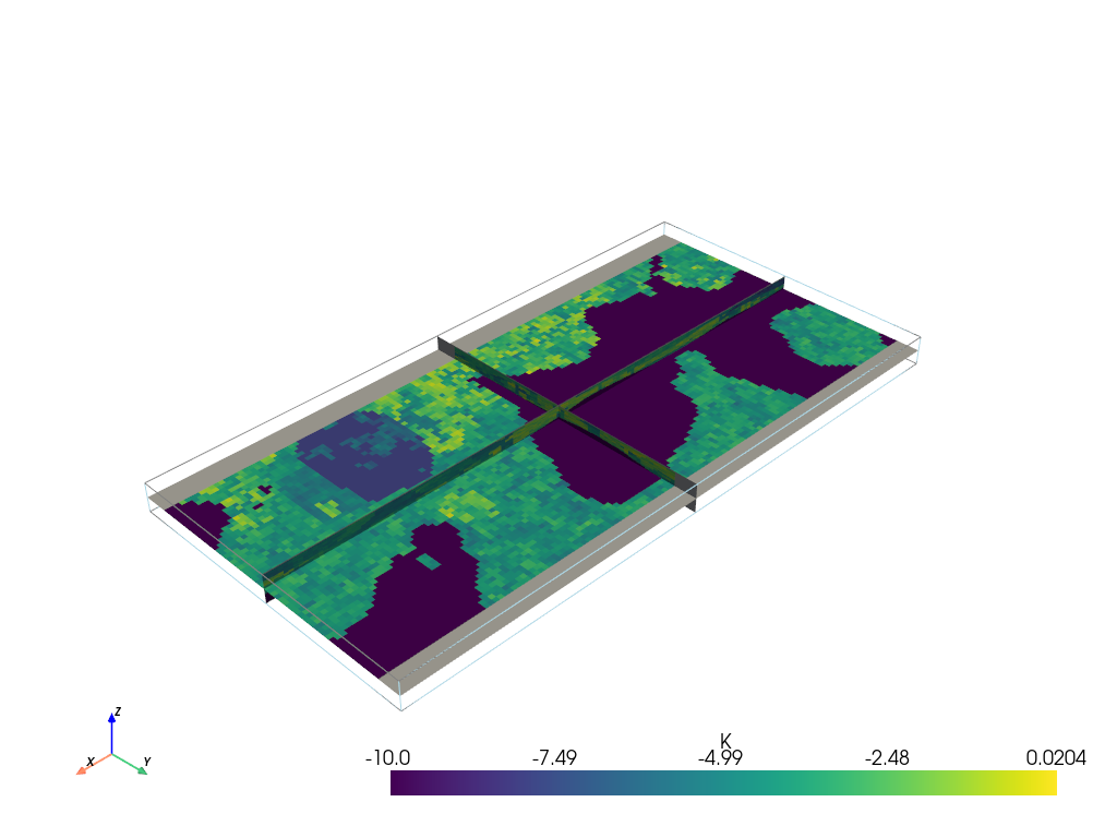
[32]:
T1.plot_prop(permea.name, 0, slicex=0.5,slicey=0.5,slicez=0.5, v_ex=v_ex)
[33]:
#property values can be retrieve with getprop method
K = T1.get_prop("K")
[34]:
#check HD
for x,y,z in x_hd:
    idx = T1.coord2cell(x, y, z)
    if idx is not None:
        print(K[2,0,0][idx])

#Some results are not respected (-10) due to the homogenous method applied on A unit
point outside of the grid in x
[35]:
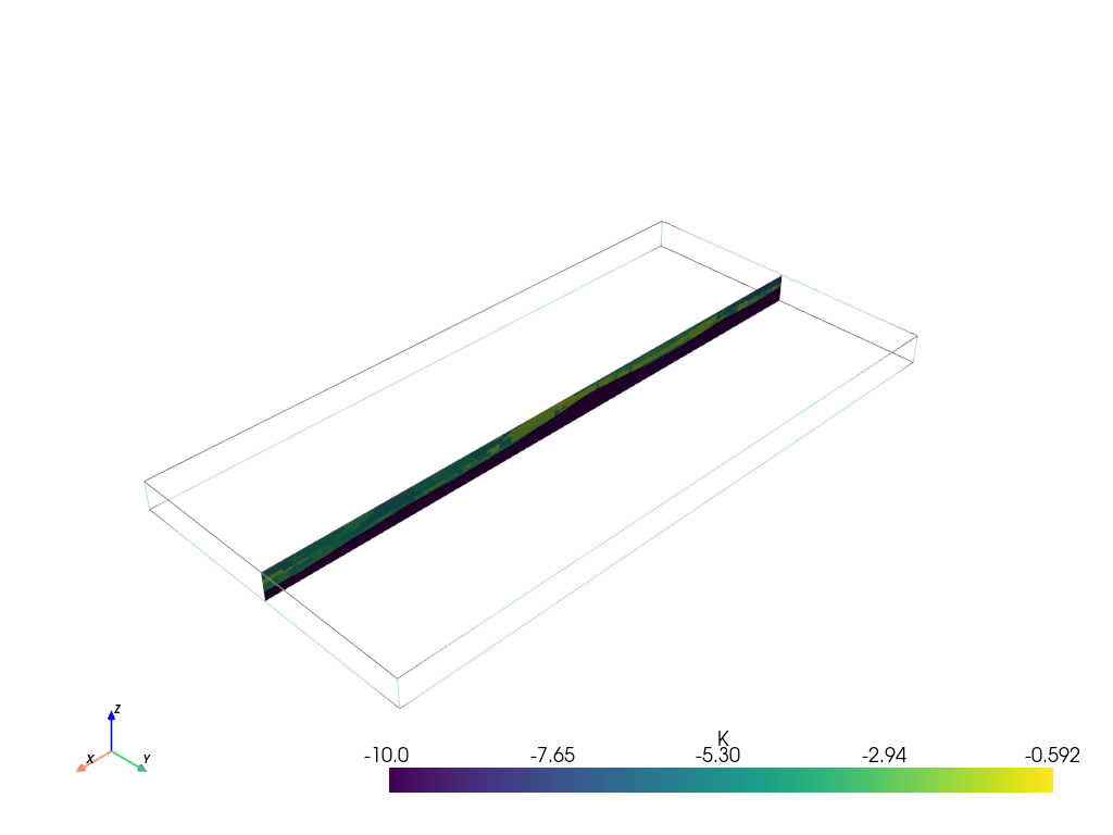
T1.plot_mean_prop("K", slicey = 0.5)
[36]:
ArchPy.inputs.save_project(T1)
Warning: Flag argument of unit D is possibly not compatible with the export
Project saved successfully
[36]:
True
[37]:
for i in T1.list_props[0].x:

    if hasattr(i, "__iter__"):
        print([float(o) for o in i])
[0.0, 5.0, -10.0]
[1.5, 5.0, -10.0]
[3.0, 5.0, -10.0]
[4.5, 5.0, -10.0]
[6.0, 5.0, -10.0]
[7.5, 5.0, -10.0]
[9.0, 5.0, -10.0]
[10.5, 5.0, -10.0]
[12.0, 5.0, -10.0]
[13.5, 5.0, -10.0]
[15.0, 5.0, -10.0]
[16.5, 5.0, -10.0]
[18.0, 5.0, -10.0]
[19.5, 5.0, -10.0]
[21.0, 5.0, -10.0]
[22.5, 5.0, -10.0]
[24.0, 5.0, -10.0]
[25.5, 5.0, -10.0]
[27.0, 5.0, -10.0]
[28.5, 5.0, -10.0]
[30.0, 5.0, -10.0]
[31.5, 5.0, -10.0]
[33.0, 5.0, -10.0]
[34.5, 5.0, -10.0]
[36.0, 5.0, -10.0]
[37.5, 5.0, -10.0]
[39.0, 5.0, -10.0]
[40.5, 5.0, -10.0]
[42.0, 5.0, -10.0]
[43.5, 5.0, -10.0]
[45.0, 5.0, -10.0]
[46.5, 5.0, -10.0]
[48.0, 5.0, -10.0]
[49.5, 5.0, -10.0]
[51.0, 5.0, -10.0]
[52.5, 5.0, -10.0]
[54.0, 5.0, -10.0]
[55.5, 5.0, -10.0]
[57.0, 5.0, -10.0]
[58.5, 5.0, -10.0]
[60.0, 5.0, -10.0]
[61.5, 5.0, -10.0]
[63.0, 5.0, -10.0]
[64.5, 5.0, -10.0]
[66.0, 5.0, -10.0]
[67.5, 5.0, -10.0]
[69.0, 5.0, -10.0]
[70.5, 5.0, -10.0]
[72.0, 5.0, -10.0]
[73.5, 5.0, -10.0]
[75.0, 5.0, -10.0]
[76.5, 5.0, -10.0]
[78.0, 5.0, -10.0]
[79.5, 5.0, -10.0]
[81.0, 5.0, -10.0]
[82.5, 5.0, -10.0]
[84.0, 5.0, -10.0]
[85.5, 5.0, -10.0]
[87.0, 5.0, -10.0]
[88.5, 5.0, -10.0]
[90.0, 5.0, -10.0]
[91.5, 5.0, -10.0]
[93.0, 5.0, -10.0]
[94.5, 5.0, -10.0]
[96.0, 5.0, -10.0]
[97.5, 5.0, -10.0]
[99.0, 5.0, -10.0]
[100.5, 5.0, -10.0]
[102.0, 5.0, -10.0]
[103.5, 5.0, -10.0]
[105.0, 5.0, -10.0]
[106.5, 5.0, -10.0]
[108.0, 5.0, -10.0]
[109.5, 5.0, -10.0]
[111.0, 5.0, -10.0]
[112.5, 5.0, -10.0]
[114.0, 5.0, -10.0]
[115.5, 5.0, -10.0]
[117.0, 5.0, -10.0]
[118.5, 5.0, -10.0]
[120.0, 5.0, -10.0]
[121.5, 5.0, -10.0]
[123.0, 5.0, -10.0]
[124.5, 5.0, -10.0]
[126.0, 5.0, -10.0]
[127.5, 5.0, -10.0]
[129.0, 5.0, -10.0]
[130.5, 5.0, -10.0]
[132.0, 5.0, -10.0]
[133.5, 5.0, -10.0]
[135.0, 5.0, -10.0]
[136.5, 5.0, -10.0]
[138.0, 5.0, -10.0]
[139.5, 5.0, -10.0]
[141.0, 5.0, -10.0]
[142.5, 5.0, -10.0]
[144.0, 5.0, -10.0]
[145.5, 5.0, -10.0]
[147.0, 5.0, -10.0]
[148.5, 5.0, -10.0]
[150.0, 5.0, -10.0]
[151.5, 5.0, -10.0]
[153.0, 5.0, -10.0]
[154.5, 5.0, -10.0]
[156.0, 5.0, -10.0]
[157.5, 5.0, -10.0]
[159.0, 5.0, -10.0]
[160.5, 5.0, -10.0]
[162.0, 5.0, -10.0]
[163.5, 5.0, -10.0]
[165.0, 5.0, -10.0]
[166.5, 5.0, -10.0]
[168.0, 5.0, -10.0]
[169.5, 5.0, -10.0]
[171.0, 5.0, -10.0]
[172.5, 5.0, -10.0]
[174.0, 5.0, -10.0]
[175.5, 5.0, -10.0]
[177.0, 5.0, -10.0]
[178.5, 5.0, -10.0]
[180.0, 5.0, -10.0]
[181.5, 5.0, -10.0]
[183.0, 5.0, -10.0]
[184.5, 5.0, -10.0]
[186.0, 5.0, -10.0]
[187.5, 5.0, -10.0]
[189.0, 5.0, -10.0]
[190.5, 5.0, -10.0]
[192.0, 5.0, -10.0]
[193.5, 5.0, -10.0]
[195.0, 5.0, -10.0]
[196.5, 5.0, -10.0]
[198.0, 5.0, -10.0]