ArchPy2Modflow: paper examples
[1]:
import numpy as np
import pandas as pd
import matplotlib
from matplotlib import colors
import matplotlib.pyplot as plt
import geone
import geone.covModel as gcm
import geone.imgplot3d as imgplt3
import pyvista as pv
import sys
import os

# auto reload modules
%load_ext autoreload
%autoreload 2

sys.path.append("../../")

#my modules
from ArchPy.base import *
from ArchPy.tpgs import *
[2]:
#grid
sx = 1.5
sy = 1.5
sz = .15
x0 = 0
y0 = 0
z0 = -15
nx = 100
ny = 50
nz = 50
x1 = x0 + nx*sx
y1 = y0 + ny*sy
z1 = z0 + nz*sz

dimensions = (nx, ny, nz)
spacing = (sx, sy, sz)
origin = (x0, y0, z0)
[3]:
## create pile

P1 = Pile(name = "P1",seed=1)

#units covmodel
covmodelD = gcm.CovModel2D(elem=[('cubic', {'w':0.6, 'r':[30,30]})])
covmodelD1 = gcm.CovModel2D(elem=[('cubic', {'w':0.2, 'r':[30,30]})])
covmodelC = gcm.CovModel2D(elem=[('cubic', {'w':0.2, 'r':[40,40]})])
covmodelB = gcm.CovModel2D(elem=[('cubic', {'w':0.6, 'r':[30,30]})])
covmodel_er = gcm.CovModel2D(elem=[('spherical', {'w':1, 'r':[50,50]})])

# facies covmodels
covmodel_f_B_gravel = gcm.CovModel3D(elem=[('spherical', {'w':0.6*0.4, 'r':[20, 20, 2]})])
covmodel_f_B_sand = gcm.CovModel3D(elem=[('spherical', {'w':0.3*0.7, 'r':[20, 20, 2]})])
covmodel_f_B_clay = gcm.CovModel3D(elem=[('spherical', {'w':0.1*0.9, 'r':[30, 30, 0.5]})])

#create Lithologies
dic_s_D = {"int_method" : "grf_ineq","covmodel" : covmodelD}
dic_f_D = {"f_method":"homogenous"}
D = Unit(name="D",order=1,ID = 1,color="gold",contact="onlap",surface=Surface(contact="onlap",dic_surf=dic_s_D)
         ,dic_facies=dic_f_D)

dic_s_C = {"int_method" : "grf_ineq","covmodel" : covmodelC, "mean":-8.5}
dic_f_C = {"f_method":"homogenous"}
C = Unit(name="C", order=2, ID = 2, color="blue", contact="onlap", dic_facies=dic_f_C, surface=Surface(dic_surf=dic_s_C, contact="onlap"))

dic_s_B = {"int_method" : "grf_ineq","covmodel" : covmodelB, "mean":-9.5}
dic_f_B = {"f_method":"SIS", "f_covmodel":[covmodel_f_B_sand, covmodel_f_B_gravel, covmodel_f_B_clay], "probability":[0.3, 0.6, 0.1]}
B = Unit(name="B",order=3,ID = 3,color="violet",contact="onlap",dic_facies=dic_f_B,surface=Surface(contact="onlap",dic_surf=dic_s_B))

dic_s_A = {"int_method":"grf_ineq","covmodel": covmodelB, "mean":-13}
dic_f_A = {"f_method":"homogenous"}
A = Unit(name="A",order=4, ID = 4,color="red",contact="onlap",dic_facies=dic_f_A,surface=Surface(dic_surf = dic_s_A,contact="onlap"))

#Master pile
P1.add_unit([D,C,B,A])
Unit D: Surface added for interpolation
Unit C: Surface added for interpolation
Unit B: Surface added for interpolation
Unit A: Surface added for interpolation
Stratigraphic unit D added ✅
Stratigraphic unit C added ✅
Stratigraphic unit B added ✅
Stratigraphic unit A added ✅
[4]:
# covmodels for the property model
covmodelK = gcm.CovModel3D(elem=[("exponential",{"w":0.3,"r":[30,30,10]})],alpha=-20,name="K_vario")
covmodelK2 = gcm.CovModel3D(elem=[("spherical",{"w":0.1,"r":[20,20, 5]})],alpha=0,name="K_vario_2")

facies_1 = Facies(ID = 1,name="Sand",color="yellow")
facies_2 = Facies(ID = 2,name="Gravel",color="lightgreen")
facies_4 = Facies(ID = 4,name="Clay",color="blue")
facies_7 = Facies(ID = 7,name="basement",color="red")

A.add_facies([facies_7])
B.add_facies([facies_1, facies_2, facies_4])
D.add_facies([facies_1])
C.add_facies([facies_4])

# property model

# K
# cm_prop1 = gcm.CovModel3D(elem = [("spherical", {"w":0.5, "r":[10, 10, 10]}),
#                                   ("cubic", {"w":0.5, "r":[15, 15, 15]})])
cm_prop2 = gcm.CovModel3D(elem = [("cubic", {"w":0.25, "r":[25, 25, 25]})])

list_facies = [facies_1, facies_2, facies_4, facies_7]
means = [-3.5, -2, -8, -10]
prop_model = ArchPy.base.Prop("K",
                              facies = list_facies,
                              covmodels = [cm_prop2, cm_prop2, cm_prop2, cm_prop2],
                                means = means,
                                int_method = ["sgs", "sgs", "sgs", "homogenous"],
                                vmin = -10,
                                vmax = -1
                                )

# porosity
cm_prop2_sand = gcm.CovModel3D(elem = [("cubic", {"w":0.005, "r":[15, 15, 15]})])
cm_prop2_gravel = gcm.CovModel3D(elem = [("cubic", {"w":0.005, "r":[15, 15, 15]})])
cm_prop2_clay = gcm.CovModel3D(elem = [("cubic", {"w":0.026, "r":[15, 15, 15]})])
cm_prop2_basement = gcm.CovModel3D(elem = [("cubic", {"w":0.0218, "r":[15, 15, 15]})])

porosity = ArchPy.base.Prop("Porosity",
                            facies = list_facies,
                            covmodels = [cm_prop2_sand, cm_prop2_gravel, cm_prop2_clay, cm_prop2_basement],
                            # means = [0.3, 0.3, 0.1, 0.05],
                            means = [-0.37, -0.37, -0.958, -1.30],
                            int_method = ["sgs", "sgs", "sgs", "homogenous"],
                            vmin = 0,
                            vmax = 0.4,
                            log_void_ratio=True
                            )

# alh
long_disp = ArchPy.base.Prop("long_disp",
                            facies = list_facies,
                            covmodels = None,
                            # means = [1.5, 1.5, 1.5, 1.5],
                            means = [10, 10, 10, 10],
                            int_method = ["homogenous", "homogenous", "homogenous", "homogenous"],
                            vmin = 0
                            )
Facies basement added to unit A ✅
Facies Sand added to unit B ✅
Facies Gravel added to unit B ✅
Facies Clay added to unit B ✅
Facies Sand added to unit D ✅
Facies Clay added to unit C ✅
[5]:
porosity.log_void_ratio
[5]:
True
[6]:
top = np.ones([ny,nx])*z1
bot = np.ones([ny,nx])*z0
[7]:
T1 = Arch_table(name = "P1",seed=1)
T1.set_Pile_master(P1)
T1.add_grid(dimensions, spacing, origin, top=top,bot=bot)
T1.add_prop([prop_model, porosity, long_disp])
Pile sets as Pile master
## Adding Grid ##
## Grid added and is now simulation grid ##
Property K added
Property Porosity added
Property long_disp added
[8]:
T1.get_sp(unit_kws=["covmodel"], facies_kws=["probability", "f_covmodel"])[0]
[8]:
| name | contact | int_method | covmodel | filling_method | list_facies | probability | f_covmodel | |
|---|---|---|---|---|---|---|---|---|
| 0 | D | onlap | grf_ineq | 0: cub (w: 0.6, r: [30, 30]) | homogenous | [Sand] | None | None |
| 1 | C | onlap | grf_ineq | 0: cub (w: 0.2, r: [40, 40]) | homogenous | [Clay] | None | None |
| 2 | B | onlap | grf_ineq | 0: cub (w: 0.6, r: [30, 30]) | SIS | [Sand, Gravel, Clay] | [0.3, 0.6, 0.1] | Sand : 0: sph (w: 0.21, r: [20, 20, 2]) | Gravel : 0: sph (w: 0.24, r: [20, 20, 2]) | Clay : 0: sph (w: 0.09000000000000001, r: [30, 30, 0.5]) | |
| 3 | A | onlap | grf_ineq | 0: cub (w: 0.6, r: [30, 30]) | homogenous | [basement] | None | None |
[9]:
T1.get_sp()[1]
[9]:
| name | property | mean | covmodels | |
|---|---|---|---|---|
| 0 | Sand | K | -3.500000 | 0: cub (w: 0.25, r: [25, 25, 25]) |
| 1 | Sand | Porosity | -0.370000 | 0: cub (w: 0.005, r: [15, 15, 15]) |
| 2 | Sand | long_disp | 10.000000 | None |
| 3 | Clay | K | -8.000000 | 0: cub (w: 0.25, r: [25, 25, 25]) |
| 4 | Clay | Porosity | -0.958000 | 0: cub (w: 0.026, r: [15, 15, 15]) |
| 5 | Clay | long_disp | 10.000000 | None |
| 6 | Gravel | K | -2.000000 | 0: cub (w: 0.25, r: [25, 25, 25]) |
| 7 | Gravel | Porosity | -0.370000 | 0: cub (w: 0.005, r: [15, 15, 15]) |
| 8 | Gravel | long_disp | 10.000000 | None |
| 9 | basement | K | -10.000000 | 0: cub (w: 0.25, r: [25, 25, 25]) |
| 10 | basement | Porosity | -1.300000 | 0: cub (w: 0.0218, r: [15, 15, 15]) |
| 11 | basement | long_disp | 10.000000 | None |
[10]:
T1.compute_surf(1)
T1.compute_facies(1)
T1.compute_prop(1)
Boreholes not processed, fully unconditional simulations will be tempted
########## PILE P1 ##########
Pile P1: ordering units
Stratigraphic units have been sorted according to order

#### COMPUTING SURFACE OF UNIT A
A: time elapsed for computing surface 0.22097539901733398 s

#### COMPUTING SURFACE OF UNIT B
B: time elapsed for computing surface 0.06750726699829102 s

#### COMPUTING SURFACE OF UNIT C
C: time elapsed for computing surface 0.06752967834472656 s

#### COMPUTING SURFACE OF UNIT D
D: time elapsed for computing surface 0.0 s

Time elapsed for getting domains 0.008999824523925781 s
##########################


### 0.37401270866394043: Total time elapsed for computing surfaces ###

### Unit D: facies simulation with homogenous method ####
### Unit D - realization 0 ###
Time elapsed 0.0 s

### Unit C: facies simulation with homogenous method ####
### Unit C - realization 0 ###
Time elapsed 0.0 s

### Unit B: facies simulation with SIS method ####
### Unit B - realization 0 ###
Time elapsed 1.67 s

### Unit A: facies simulation with homogenous method ####
### Unit A - realization 0 ###
Time elapsed 0.0 s

### 1.67: Total time elapsed for computing facies ###
### 1 K property models will be modeled ###
### 1 K models done
### 1 Porosity property models will be modeled ###
### 1 Porosity models done
### 1 long_disp property models will be modeled ###
### 1 long_disp models done
Test upscaling disp
[11]:
pv.set_jupyter_backend("static")
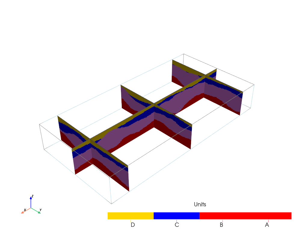
[12]:
T1.plot_units(v_ex=3, slicex=(0.1, 0.5, 0.9), slicey=0.5)
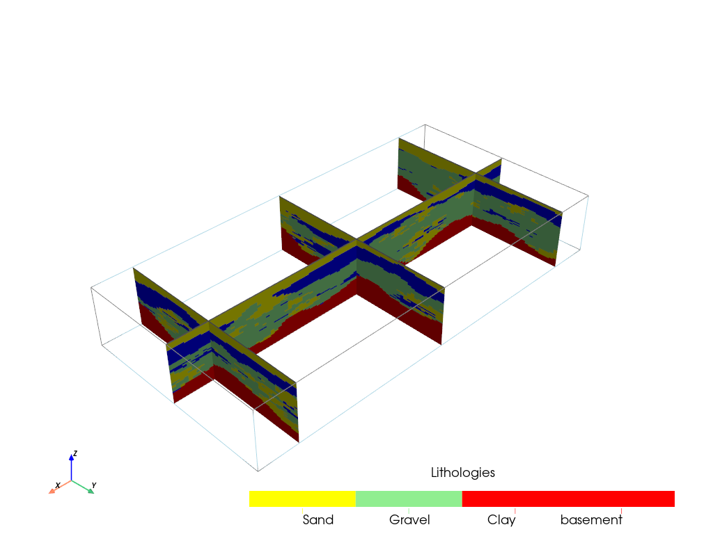
[13]:
T1.plot_facies(v_ex=3, slicex=(0.1, 0.5, 0.9), slicey=0.5)
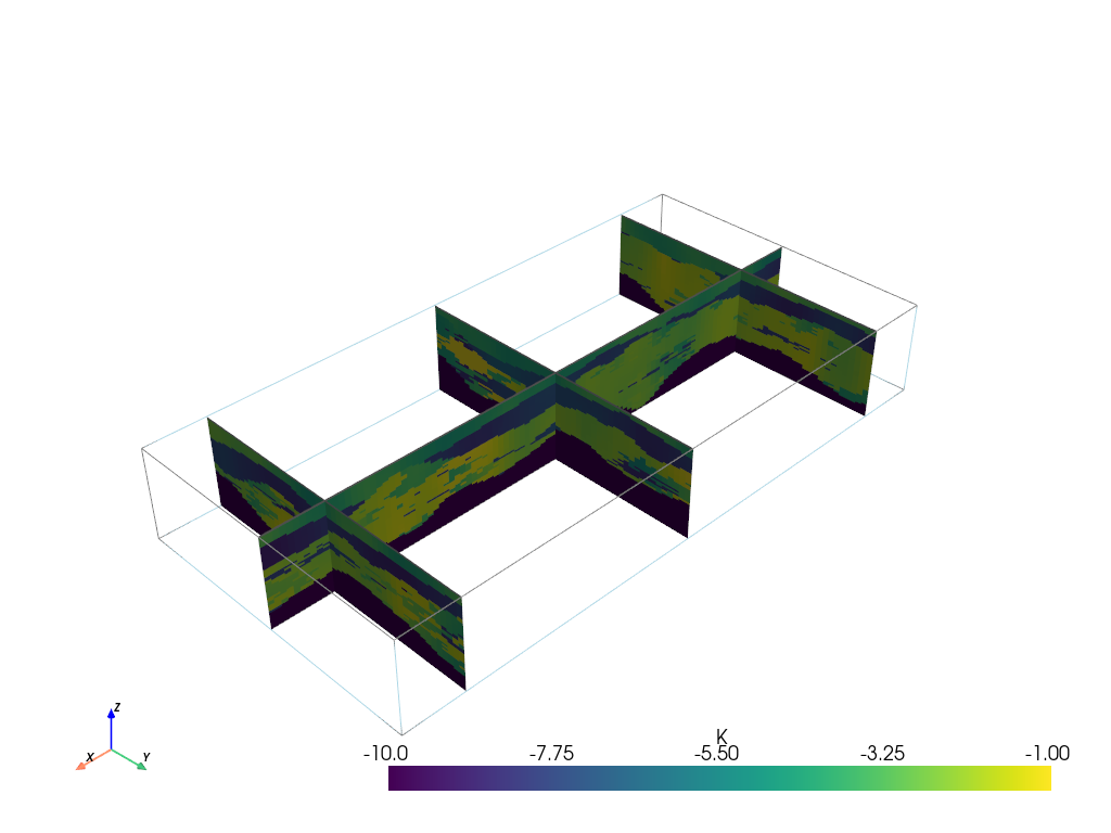
[14]:
T1.plot_prop("K", v_ex=3, slicex=(0.1, 0.5, 0.9), slicey=0.5)
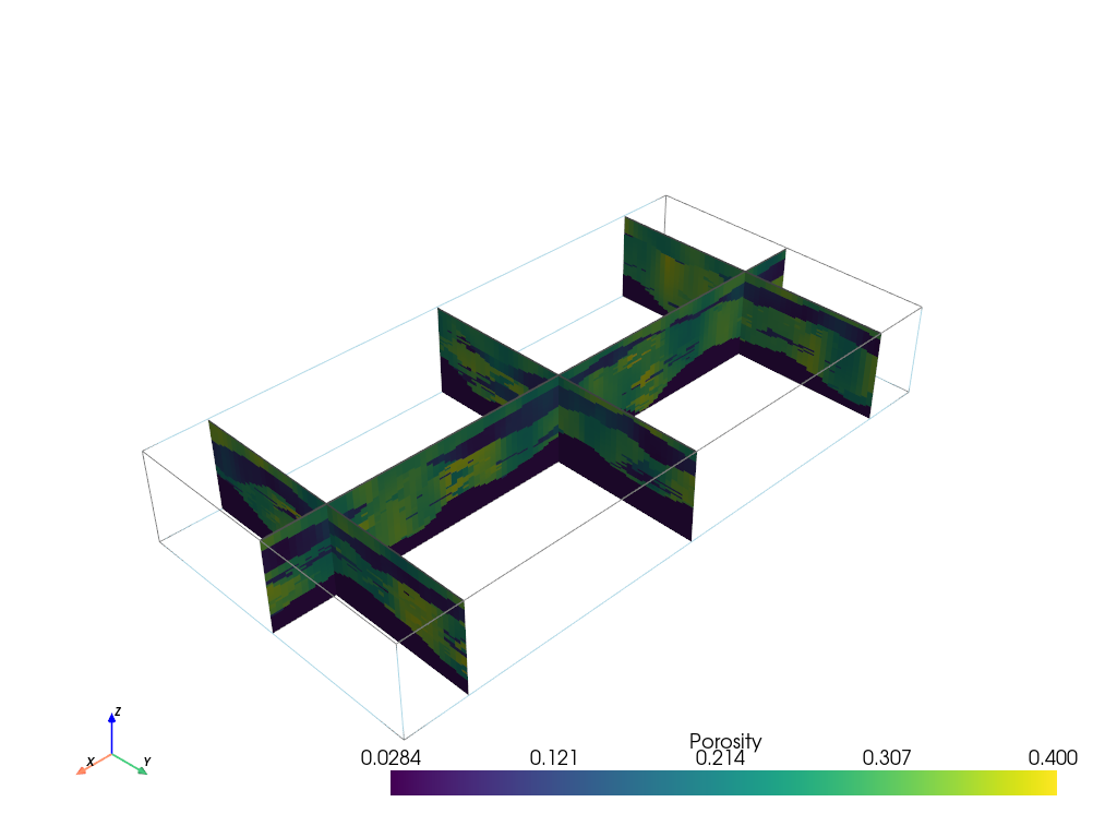
[15]:
T1.plot_prop("Porosity", v_ex=3, slicex=(0.1, 0.5, 0.9), slicey=0.5)
[16]:
# ArchPy.inputs.save_project(T1)
Heterogeneous
Flow model
[17]:
import ArchPy.ap_mf
from ArchPy.ap_mf import archpy2modflow, array2cellids
import flopy as fp
[18]:
mf6_exe_path = "../../../../exe/mf6.exe"
[58]:
archpy_flow = archpy2modflow(T1, exe_name=mf6_exe_path, model_dir="layered_hetero")  # create the modflow model
archpy_flow.create_sim(grid_mode="layers", iu=0, unit_limit=None, lay_sep=[1, 1, 3, 1], factor_x=2, factor_y=2, factor_z=2)  # create the simulation object and choose a certain discretization
Simulation created with the following parameters:
Grid mode: layers
To retrieve the simulation, use the get_sim() method
[59]:
archpy_flow.set_k("K", iu=0, ifa=0, ip=0, log=True, k_average_method="anisotropic", average_facies=True) # set the hydraulic conductivity
[60]:
sim = archpy_flow.get_sim()
gwf = archpy_flow.get_gwf()
[61]:
sim.ims.remove()
inner_dvclose = 1e-5
ims = fp.mf6.ModflowIms(sim, complexity="moderate", inner_dvclose=inner_dvclose)
[62]:
# add BC at left and right on all layers
h1 = .3
h2 = 0
T_1 = 10  # temperature at left boundary
T_2 = 10  # temperature at right boundary
chd_data = []

a = np.zeros((gwf.modelgrid.nlay, gwf.modelgrid.nrow, gwf.modelgrid.ncol), dtype=bool)
a[:, :, 0] = 1
lst_chd = array2cellids(a, gwf.dis.idomain.array)
for cellid in lst_chd:
    chd_data.append((cellid, h1, T_1))

chd1 = fp.mf6.ModflowGwfchd(gwf, stress_period_data=chd_data, save_flows=True, auxiliary="TEMPERATURE", pname="CHD-1")

chd_data = []
a = np.zeros((gwf.modelgrid.nlay, gwf.modelgrid.nrow, gwf.modelgrid.ncol), dtype=bool)
a[:, :, -1] = 1
lst_chd = array2cellids(a, gwf.dis.idomain.array)
for cellid in lst_chd:
    chd_data.append((cellid, h2, T_2))

chd2 = fp.mf6.ModflowGwfchd(gwf, stress_period_data=chd_data, save_flows=True, auxiliary="TEMPERATURE", pname="CHD-2")
[63]:
# add an injection well in the middle of the model
well_data = []
Q_well = 0.0015  # m3/s
T_well = 7  # temperature of the injected water
cellid_well = (2, T1.ny // 2, T1.nx // 2)
well_data.append((cellid_well, Q_well, T_well))
wel = fp.mf6.ModflowGwfwel(gwf, stress_period_data=well_data, save_flows=True, auxiliary="TEMPERATURE", pname="WEL-INJ")

# production well
well_data = []
Q_well = -Q_well # m3/s
cellid_well = (2, T1.ny // 2, int(T1.nx // 2.5))
well_data.append((cellid_well, Q_well))
wel = fp.mf6.ModflowGwfwel(gwf, stress_period_data=well_data, save_flows=True, pname="WEL-PROD")
[64]:
sim.write_simulation()
sim.run_simulation()
writing simulation...
  writing simulation name file...
  writing simulation tdis package...
  writing solution package ims_-1...
  writing model test...
    writing model name file...
    writing package dis...
    writing package ic...
    writing package oc...
    writing package npf...
    writing package chd-1...
INFORMATION: maxbound in ('gwf6', 'chd', 'dimensions') changed to 300 based on size of stress_period_data
    writing package chd-2...
INFORMATION: maxbound in ('gwf6', 'chd', 'dimensions') changed to 297 based on size of stress_period_data
    writing package wel-inj...
INFORMATION: maxbound in ('gwf6', 'wel', 'dimensions') changed to 1 based on size of stress_period_data
    writing package wel-prod...
INFORMATION: maxbound in ('gwf6', 'wel', 'dimensions') changed to 1 based on size of stress_period_data
FloPy is using the following executable to run the model: \\home\schorppl$\exe\mf6.exe
                                   MODFLOW 6
                U.S. GEOLOGICAL SURVEY MODULAR HYDROLOGIC MODEL
                            VERSION 6.6.1 02/10/2025

   MODFLOW 6 compiled Feb 14 2025 13:40:10 with Intel(R) Fortran Intel(R) 64
   Compiler Classic for applications running on Intel(R) 64, Version 2021.7.0
                             Build 20220726_000000

This software has been approved for release by the U.S. Geological
Survey (USGS). Although the software has been subjected to rigorous
review, the USGS reserves the right to update the software as needed
pursuant to further analysis and review. No warranty, expressed or
implied, is made by the USGS or the U.S. Government as to the
functionality of the software and related material nor shall the
fact of release constitute any such warranty. Furthermore, the
software is released on condition that neither the USGS nor the U.S.
Government shall be held liable for any damages resulting from its
authorized or unauthorized use. Also refer to the USGS Water
Resources Software User Rights Notice for complete use, copyright,
and distribution information.


 MODFLOW runs in SEQUENTIAL mode

 Run start date and time (yyyy/mm/dd hh:mm:ss): 2025/10/06 14:05:47

 Writing simulation list file: mfsim.lst
 Using Simulation name file: mfsim.nam

    Solving:  Stress period:     1    Time step:     1

 Run end date and time (yyyy/mm/dd hh:mm:ss): 2025/10/06 14:05:48
 Elapsed run time:  0.716 Seconds

 Normal termination of simulation.
[64]:
(True, [])
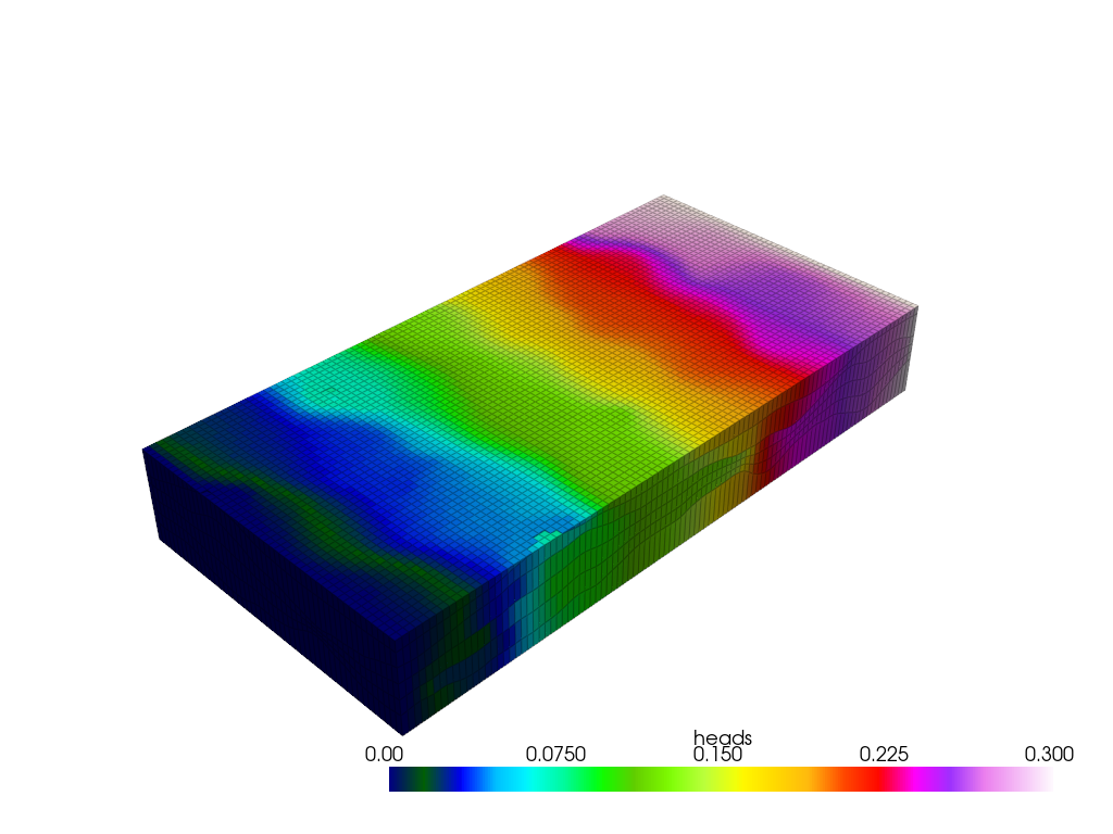
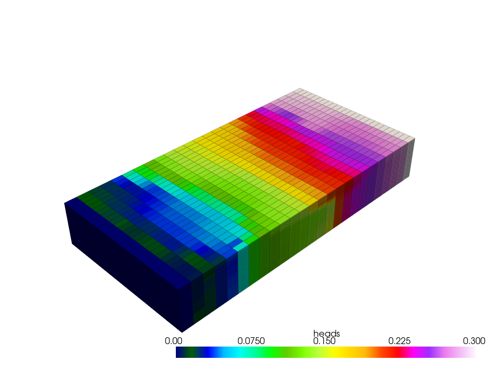
[65]:
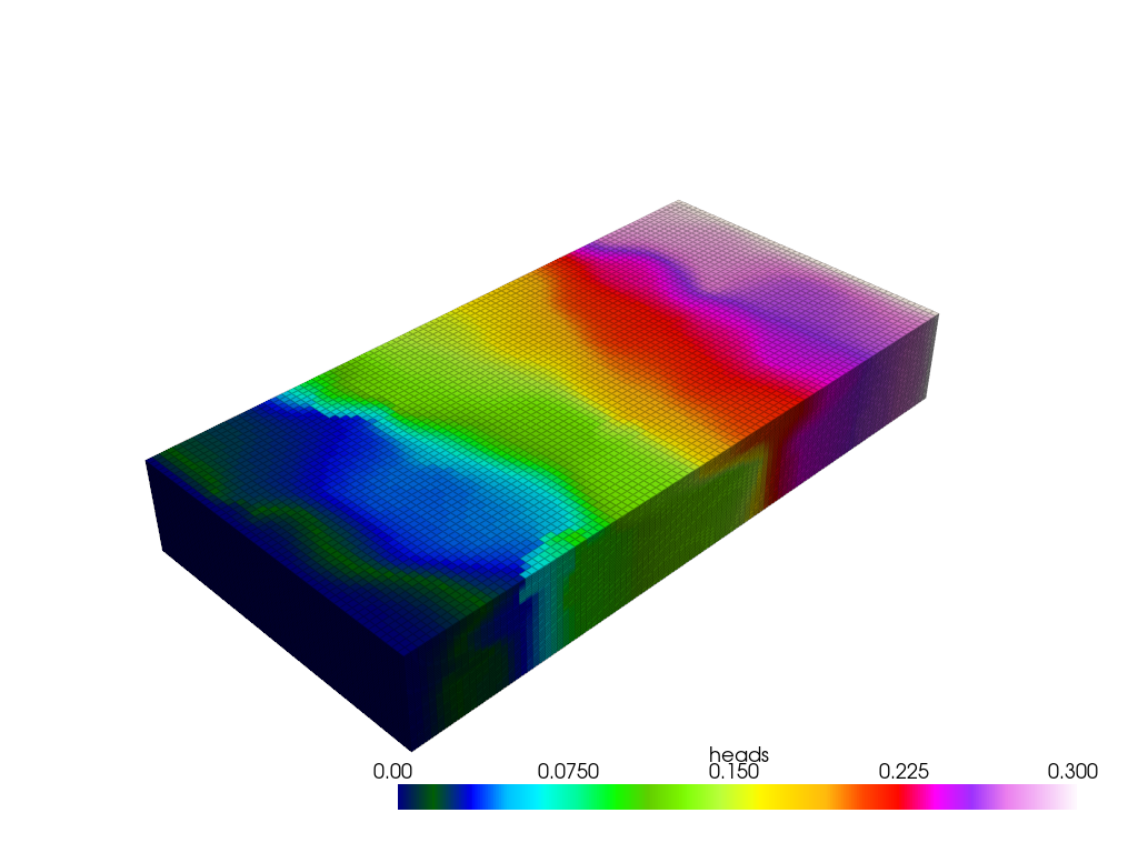
from flopy.export.vtk import Vtk

vert_exag = 3
vtk = Vtk(model=gwf, binary=False, vertical_exageration=vert_exag, smooth=True)
vtk.add_model(gwf)

# add different arrays to the vtk object
heads = archpy_flow.get_heads()
vtk.add_array(heads, name="heads")
vtk.add_array(np.log10(gwf.npf.k.array), name="K")
vtk.add_array(np.log10(gwf.npf.k33.array), name="Kzz")
vtk.add_array(gwf.npf.k.array / gwf.npf.k33.array, name="aniso")
# vtk.add_array(np.flip(archpy_flow.upscaled_facies[1], axis=1), name="prop")

gwf_mesh = vtk.to_pyvista()
ghosts = np.argwhere(gwf_mesh["idomain"] <= 0)
gwf_mesh.remove_cells(ghosts, inplace=True)

pl = pv.Plotter(notebook=True)
pl.add_mesh(gwf_mesh, opacity=1, show_edges=True, scalars="heads", cmap="gist_ncar", edge_opacity=.3, clim=[0, 0.3])

# pl.show(screenshot="../../../figures/articles/archpy 2/raw/flow_lay_he.png", window_size=[1300, 900], auto_close=False)
# pl.show(screenshot="E:/switchdrive/Post_doc/figures/articles/archpy 2/raw/flow_lay_he.png", window_size=[1300, 900], auto_close=False)
pl.show()
[66]:
heads = archpy_flow.get_heads()
[67]:
# default font size
matplotlib.rcParams.update({'font.size': 20})
[68]:
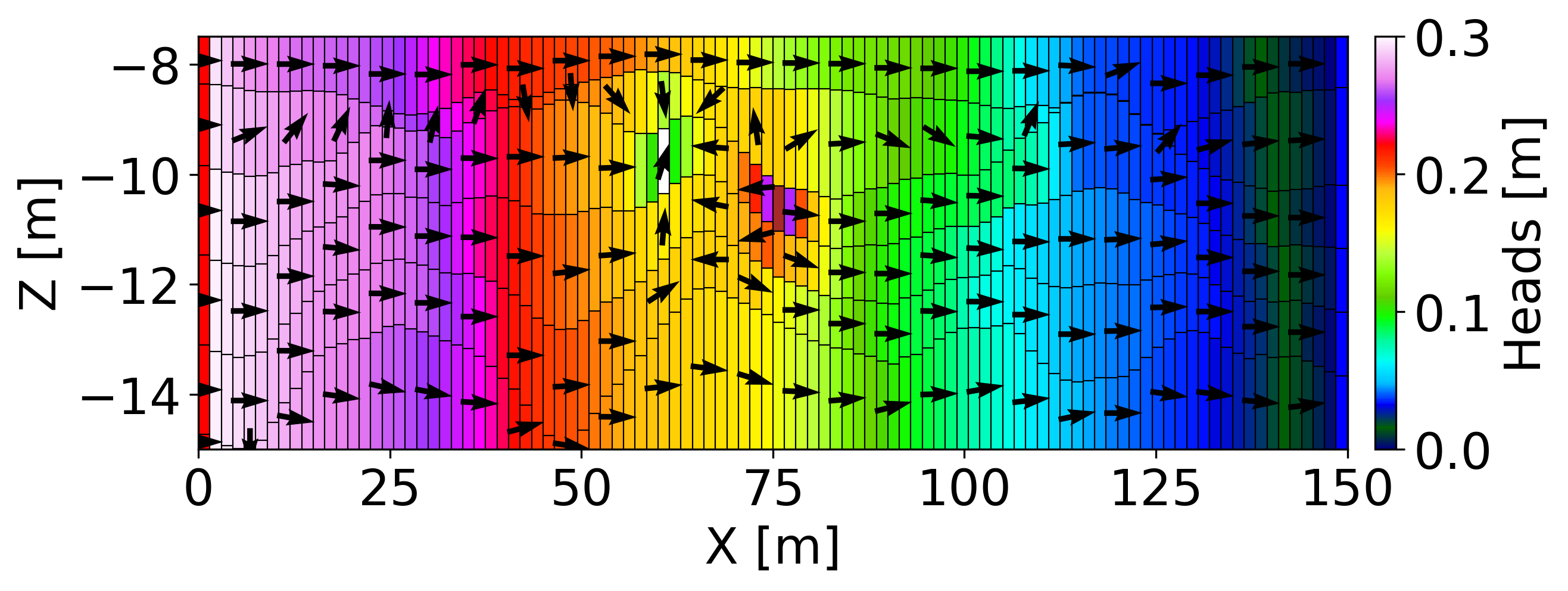
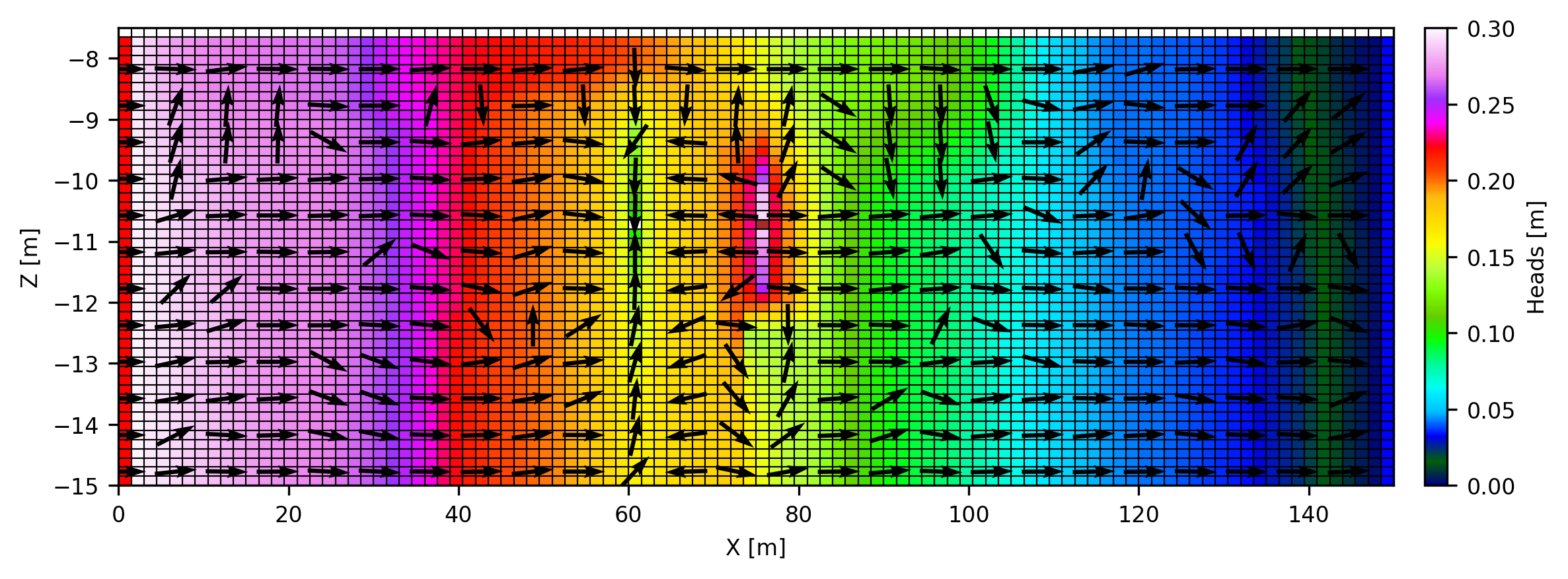
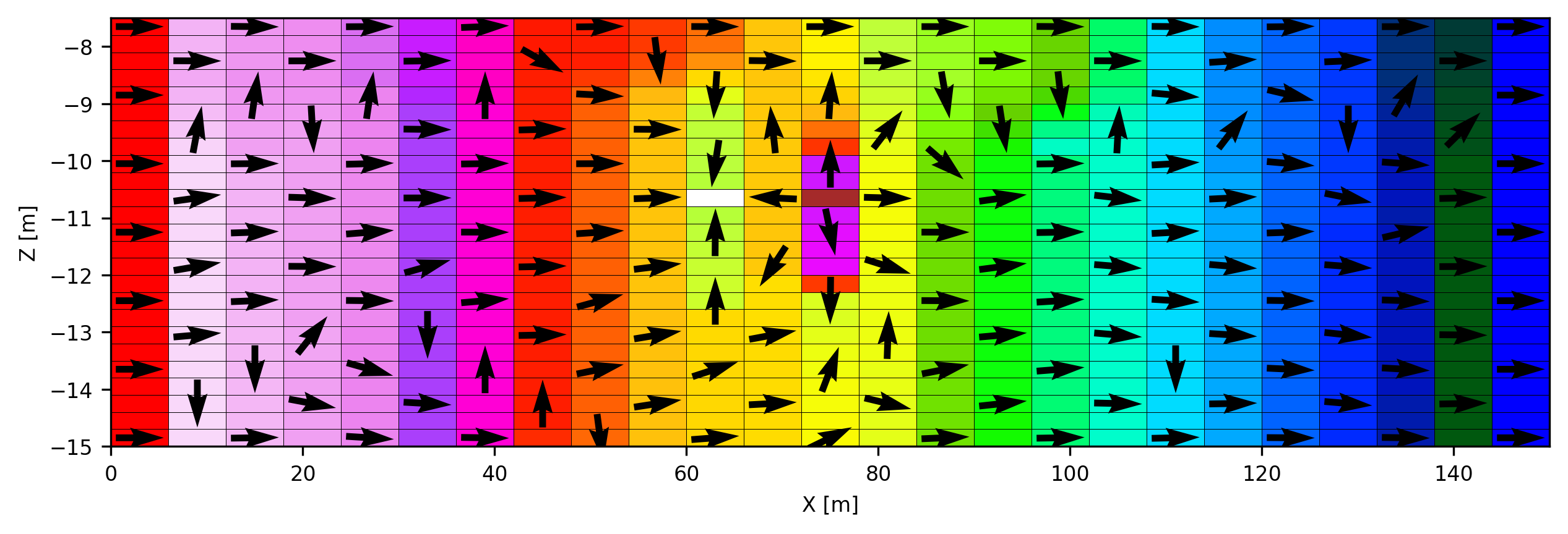
cobj = gwf.output.budget()
qx, qy, qz = fp.utils.postprocessing.get_specific_discharge(
        cobj.get_data(text="DATA-SPDIS", kstpkper=(0, 0))[0], gwf)

# plot cross section
from flopy.plot import PlotCrossSection
fig, ax = plt.subplots(1, 1, figsize=(10, 3), dpi=300)
cross_section = PlotCrossSection(model=gwf, line={"row": 25})
# cross_section.plot_array(np.log10(gwf.npf.k.array), cmap="Blues", ax=ax)
cont = cross_section.plot_array(heads, cmap="gist_ncar", ax=ax, vmin=0, vmax=0.3)
# cont = cross_section.contour_array(heads, ax=ax, levels=np.arange(0, 0.25, 0.02), linewidths=3)
# plt.clabel(cont, inline=True, fontsize=20, fmt="%.2f", colors="black")
cross_section.plot_bc("CHD-1", color="red", ax=ax)
cross_section.plot_bc("CHD-2", color="blue", ax=ax)
cross_section.plot_bc("WEL-INJ", color="brown", ax=ax)
cross_section.plot_bc("WEL-PROD", color="white", ax=ax)
cross_section.plot_vector(qx, qy, qz, color="black", normalize=True, hstep=4, kstep=1, ax=ax, scale=30)
cross_section.plot_grid(linewidth=0.5, color="black")
plt.colorbar(cont, ax=ax, label="Heads [m]", orientation="vertical", pad=0.02)
plt.xlabel("X [m]")
plt.ylabel("Z [m]")

# fig.savefig("E:/switchdrive/Post_doc/figures/articles/archpy 2/raw/flow_lay_he_cross_section.png", dpi=300, bbox_inches="tight")
[68]:
Text(0, 0.5, 'Z [m]')
[69]:
np.random.seed(15)
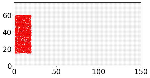
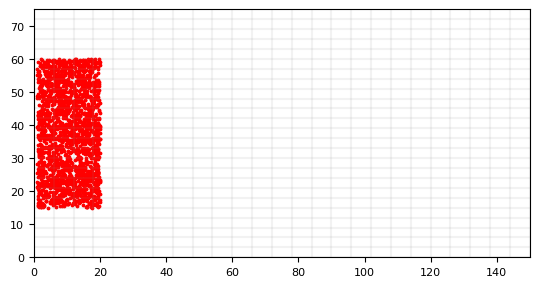
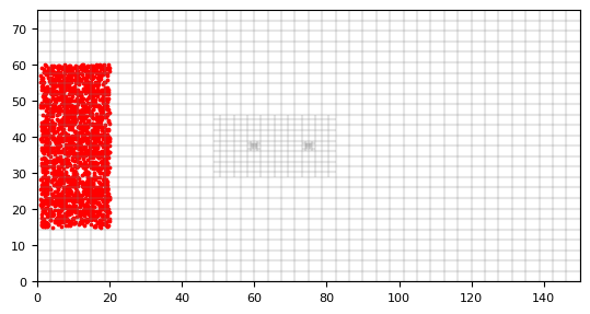
[70]:
n = 2000
xp = np.random.uniform(1, 20, n)
yp = np.random.uniform(T1.yg[-1]*0.2 + T1.yg[0], T1.yg[-1]*0.8, n)
zp = np.random.uniform(-9, -11, n)
list_p_coords = []
for i in range(n):
    list_p_coords.append((xp[i], yp[i], zp[i]))
plt.scatter(xp, yp, c="red", s=3)
gwf.modelgrid.plot(alpha=.1)
[70]:
<matplotlib.collections.LineCollection at 0x1d5214d29c0>
[71]:
archpy_flow.prt_create(prt_name="test_prt", workspace="ws_prt", trackdir="forward", list_p_coords=list_p_coords)
archpy_flow.set_porosity(prop_key="Porosity", iu=0, ifa=0, ip=0)
archpy_flow.prt_run(silent=False)
c:\Users\schorppl\.conda\envs\archpy_work\Lib\site-packages\flopy\utils\gridintersect.py:123: DeprecationWarning: Note `method="structured"` is deprecated. Pass `method="vertex"` to silence this warning. This will be the new default in a future release and this keyword argument will be removed.
  warnings.warn(
writing simulation...
  writing simulation name file...
  writing simulation tdis package...
  writing solution package ems...
  writing model test_prt...
    writing model name file...
    writing package mip...
    writing package dis...
    writing package prp...
    writing package oc...
    writing package fmi...
FloPy is using the following executable to run the model: \\home\schorppl$\exe\mf6.exe
                                   MODFLOW 6
                U.S. GEOLOGICAL SURVEY MODULAR HYDROLOGIC MODEL
                            VERSION 6.6.1 02/10/2025

   MODFLOW 6 compiled Feb 14 2025 13:40:10 with Intel(R) Fortran Intel(R) 64
   Compiler Classic for applications running on Intel(R) 64, Version 2021.7.0
                             Build 20220726_000000

This software has been approved for release by the U.S. Geological
Survey (USGS). Although the software has been subjected to rigorous
review, the USGS reserves the right to update the software as needed
pursuant to further analysis and review. No warranty, expressed or
implied, is made by the USGS or the U.S. Government as to the
functionality of the software and related material nor shall the
fact of release constitute any such warranty. Furthermore, the
software is released on condition that neither the USGS nor the U.S.
Government shall be held liable for any damages resulting from its
authorized or unauthorized use. Also refer to the USGS Water
Resources Software User Rights Notice for complete use, copyright,
and distribution information.


 MODFLOW runs in SEQUENTIAL mode

 Run start date and time (yyyy/mm/dd hh:mm:ss): 2025/10/06 14:05:58

 Writing simulation list file: mfsim.lst
 Using Simulation name file: mfsim.nam

    Solving:  Stress period:     1    Time step:     1

 Run end date and time (yyyy/mm/dd hh:mm:ss): 2025/10/06 14:06:00
 Elapsed run time:  1.867 Seconds

 Normal termination of simulation.
[72]:
df_all = archpy_flow.prt_get_pathlines()
[73]:
plt.style.use('seaborn-v0_8-pastel')
[74]:
# default font size
matplotlib.rcParams.update({'font.size': 8})
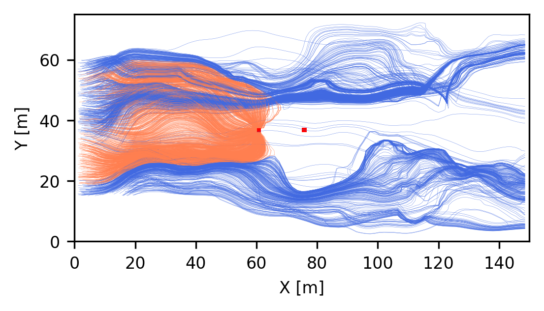
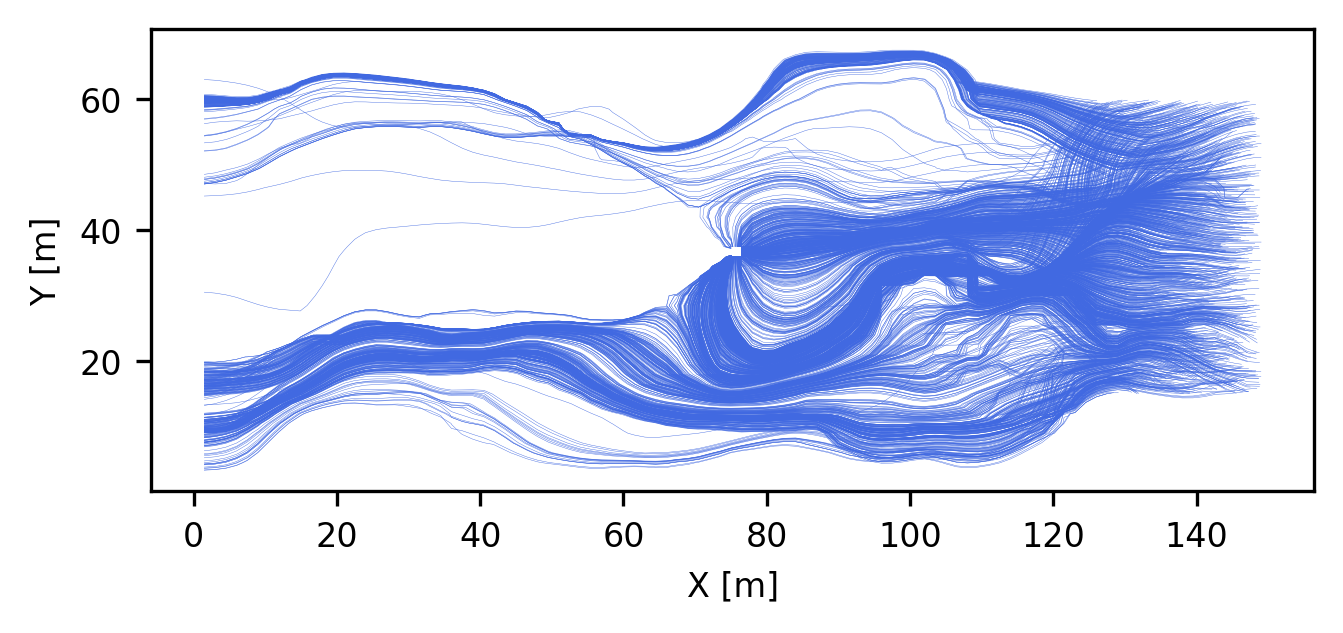
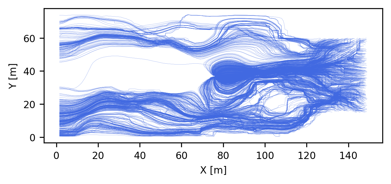
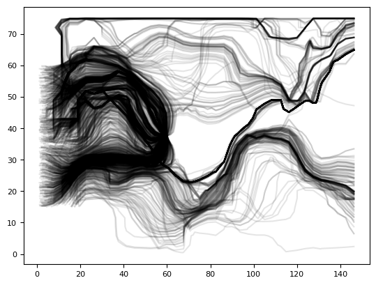
[75]:
plt.figure(figsize=(5, 2), dpi=300)

ml = fp.plot.PlotMapView(model=gwf, layer=2)
ml.plot_bc("WEL")
for i in range(1, 2000):
    xmax = df_all.loc[df_all.irpt==i].iloc[-1].x
    path = df_all.loc[df_all.irpt == i]
    if xmax < 65:
        plt.plot(path["x"], path["y"], linewidth=.1, color="coral")
    else:
        plt.plot(path["x"], path["y"], linewidth=.1, color="royalblue")


plt.xlabel("X [m]")
plt.ylabel("Y [m]")
[75]:
Text(0, 0.5, 'Y [m]')
[76]:
plt.figure(figsize=(5, 2), dpi=300)

# gwf.modelgrid.plot(alpha=.1)
for i in range(1, 2000):
    xmax = df_all.loc[df_all.irpt==i].iloc[-1].x
    path = df_all.loc[df_all.irpt == i]
    if xmax < 65:
        plt.plot(path["x"], path["z"], linewidth=.1, color="coral")
    else:
        plt.plot(path["x"], path["z"], linewidth=.1, color="royalblue")
plt.xlabel("X [m]")
plt.ylabel("Z [m]")
plt.grid()

[77]:
t_well_layhe = []
t_bc_layhe = []
for i in range(1, 2000):
    xmax = df_all.loc[df_all.irpt==i].iloc[-1].x
    if xmax < 65:
        t_well_layhe.append(df_all.loc[df_all.irpt==i].iloc[-1].t)
    else:
        t_bc_layhe.append(df_all.loc[df_all.irpt==i].iloc[-1].t)

t_well_layhe = np.array(t_well_layhe)
t_bc_layhe = np.array(t_bc_layhe)
np.save("t_well_layhe.npy", t_well_layhe)
np.save("t_bc_layhe.npy", t_bc_layhe)
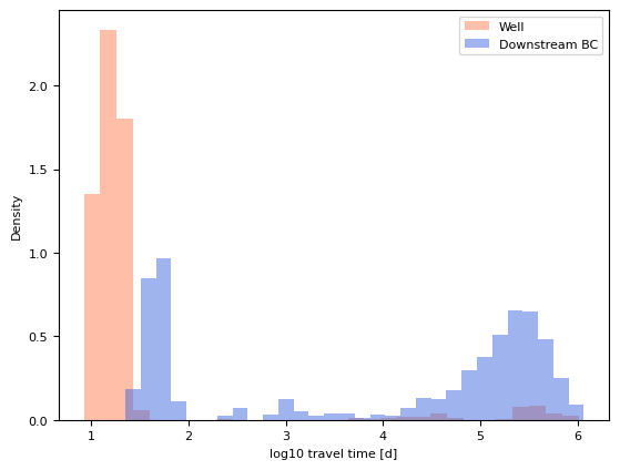
[78]:
plt.hist(np.log10(t_well_layhe / 86400), density=True, alpha=.5, label="Well", color="coral", bins=30)
plt.hist(np.log10(t_bc_layhe / 86400), density=True, alpha=.5, label="Downstream BC", color="royalblue", bins=30)

plt.xlabel("log10 travel time [d]")
plt.ylabel("Density")

plt.legend()
[78]:
<matplotlib.legend.Legend at 0x1d52aa3f350>
[79]:
import ArchPy.ap_mf
# default font size
matplotlib.rcParams.update({'font.size': 8})
[81]:
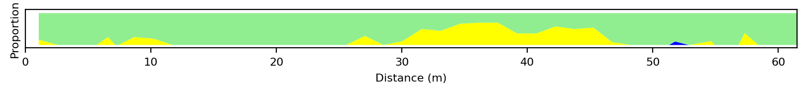
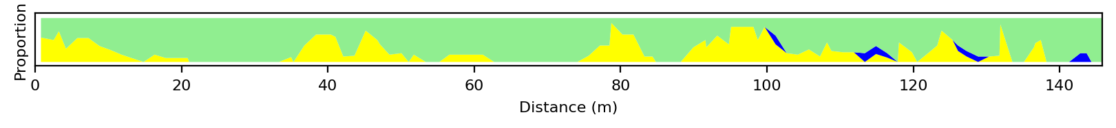
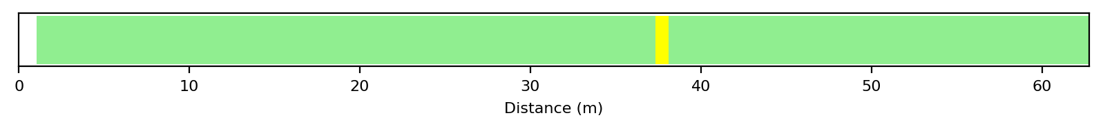
df_p = archpy_flow.prt_get_facies_path_particle(1426, facies_archpy=True)
ArchPy.ap_mf.plot_particle_facies_sequence(T1, df=df_p, plot_distance=True, proportions=False, plot_time=False)

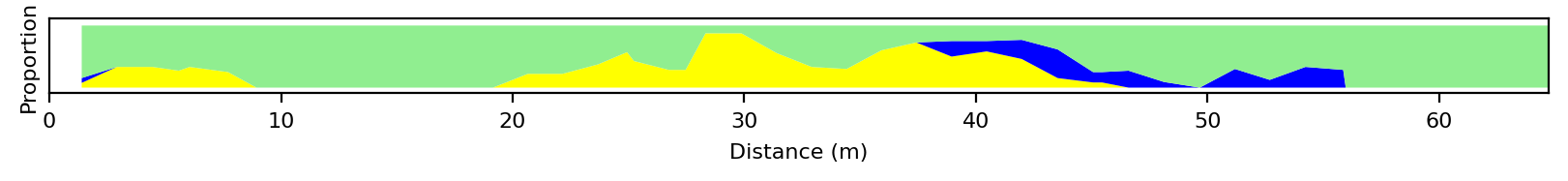
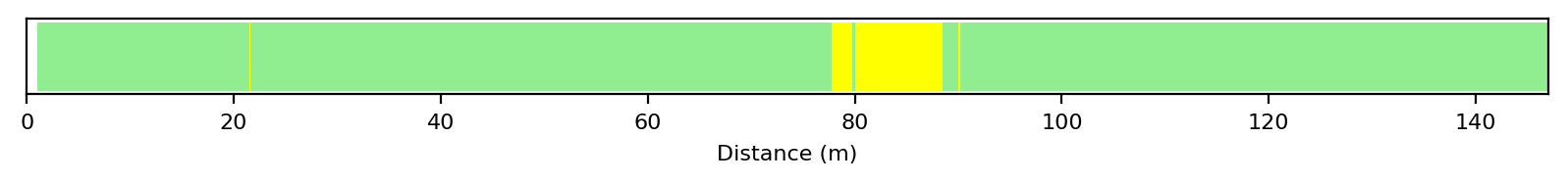
[82]:
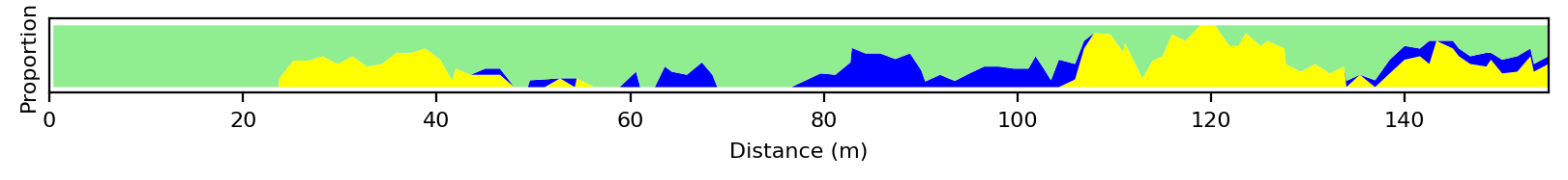
df_p = archpy_flow.prt_get_facies_path_particle(1426)
ArchPy.ap_mf.plot_particle_facies_sequence(T1, df=df_p, plot_distance=True, proportions=True, plot_time=False)

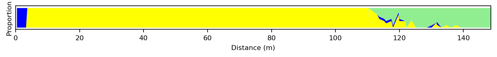
[83]:
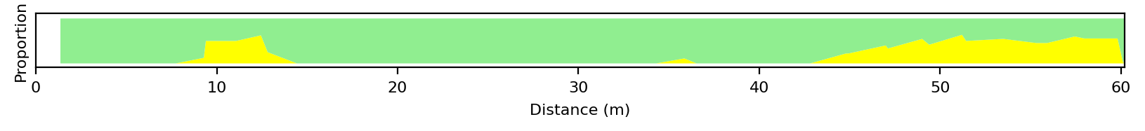
np.random.seed(1312)
for i in range(10):
    ip = np.random.randint(2000)
    df_p = archpy_flow.prt_get_facies_path_particle(ip)
    ArchPy.ap_mf.plot_particle_facies_sequence(T1, df=df_p, plot_distance=True, proportions=True, plot_time=False)


[84]:
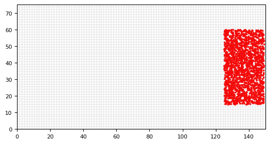
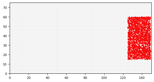
n = 2000
xp = np.random.uniform(125, 149, n)
yp = np.random.uniform(T1.yg[-1]*0.2 + T1.yg[0], T1.yg[-1]*0.8, n)
zp = np.random.uniform(-9, -11, n)
list_p_coords = []
for i in range(n):
    list_p_coords.append((xp[i], yp[i], zp[i]))
plt.scatter(xp, yp, c="red", s=3)
gwf.modelgrid.plot(alpha=.1)
[84]:
<matplotlib.collections.LineCollection at 0x1d57eeacfe0>
[85]:
archpy_flow.prt_create(prt_name="test_prt", workspace="ws_prt", trackdir="backward", list_p_coords=list_p_coords)
archpy_flow.set_porosity(prop_key="Porosity", iu=0, ifa=0, ip=0)
archpy_flow.prt_run(silent=False)
c:\Users\schorppl\.conda\envs\archpy_work\Lib\site-packages\flopy\utils\gridintersect.py:123: DeprecationWarning: Note `method="structured"` is deprecated. Pass `method="vertex"` to silence this warning. This will be the new default in a future release and this keyword argument will be removed.
  warnings.warn(
writing simulation...
  writing simulation name file...
  writing simulation tdis package...
  writing solution package ems...
  writing model test_prt...
    writing model name file...
    writing package mip...
    writing package dis...
    writing package prp...
    writing package oc...
    writing package fmi...
FloPy is using the following executable to run the model: \\home\schorppl$\exe\mf6.exe
                                   MODFLOW 6
                U.S. GEOLOGICAL SURVEY MODULAR HYDROLOGIC MODEL
                            VERSION 6.6.1 02/10/2025

   MODFLOW 6 compiled Feb 14 2025 13:40:10 with Intel(R) Fortran Intel(R) 64
   Compiler Classic for applications running on Intel(R) 64, Version 2021.7.0
                             Build 20220726_000000

This software has been approved for release by the U.S. Geological
Survey (USGS). Although the software has been subjected to rigorous
review, the USGS reserves the right to update the software as needed
pursuant to further analysis and review. No warranty, expressed or
implied, is made by the USGS or the U.S. Government as to the
functionality of the software and related material nor shall the
fact of release constitute any such warranty. Furthermore, the
software is released on condition that neither the USGS nor the U.S.
Government shall be held liable for any damages resulting from its
authorized or unauthorized use. Also refer to the USGS Water
Resources Software User Rights Notice for complete use, copyright,
and distribution information.


 MODFLOW runs in SEQUENTIAL mode

 Run start date and time (yyyy/mm/dd hh:mm:ss): 2025/10/06 14:08:34

 Writing simulation list file: mfsim.lst
 Using Simulation name file: mfsim.nam

    Solving:  Stress period:     1    Time step:     1

 Run end date and time (yyyy/mm/dd hh:mm:ss): 2025/10/06 14:08:36
 Elapsed run time:  1.897 Seconds

 Normal termination of simulation.
[86]:
df_all = archpy_flow.prt_get_pathlines()
[87]:
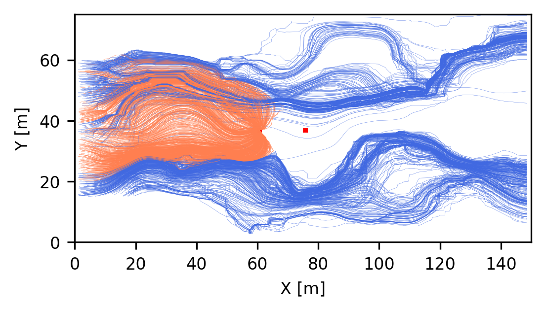
plt.figure(figsize=(5, 2), dpi=300)

# gwf.modelgrid.plot(alpha=.1)
for i in range(1, 2000):
    path = df_all.loc[df_all.irpt == i]
    plt.plot(path["x"], path["y"], linewidth=.1, color="royalblue")

plt.xlabel("X [m]")
plt.ylabel("Y [m]")
[87]:
Text(0, 0.5, 'Y [m]')
ArchPy mode - heterogeneous
[88]:
archpy_flow = archpy2modflow(T1, exe_name=mf6_exe_path, model_dir="archpy_mode_hetero")  # create the modflow model
archpy_flow.create_sim(grid_mode="archpy", iu=0, unit_limit=None)  # create the simulation object and choose a certain discretization
archpy_flow.set_k("K", iu=0, ifa=0, ip=0, log=True, k_average_method="anisotropic", average_facies=True)  # set the hydraulic conductivity
Simulation created with the following parameters:
Grid mode: archpy
To retrieve the simulation, use the get_sim() method
[89]:
sim = archpy_flow.get_sim()
gwf = archpy_flow.get_gwf()
[90]:
sim.ims.remove()
inner_dvclose = 1e-5
ims = fp.mf6.ModflowIms(sim, complexity="moderate", inner_dvclose=inner_dvclose)
[91]:
import flopy as fp
[92]:
# add BC at left and right on all layers
h1 = .3
h2 = 0
T_1 = 10  # temperature at left boundary
T_2 = 10  # temperature at right boundary
chd_data = []

a = np.zeros((gwf.modelgrid.nlay, gwf.modelgrid.nrow, gwf.modelgrid.ncol), dtype=bool)
a[:, :, 0] = 1
lst_chd = array2cellids(a, gwf.dis.idomain.array)
for cellid in lst_chd:
    chd_data.append((cellid, h1, T_1))

chd1 = fp.mf6.ModflowGwfchd(gwf, stress_period_data=chd_data, save_flows=True, auxiliary="TEMPERATURE", pname="CHD-1")

chd_data = []
a = np.zeros((gwf.modelgrid.nlay, gwf.modelgrid.nrow, gwf.modelgrid.ncol), dtype=bool)
a[:, :, -1] = 1
lst_chd = array2cellids(a, gwf.dis.idomain.array)
for cellid in lst_chd:
    chd_data.append((cellid, h2, T_2))

chd2 = fp.mf6.ModflowGwfchd(gwf, stress_period_data=chd_data, save_flows=True, auxiliary="TEMPERATURE", pname="CHD-2")
Wells at (\(75.0, 25.0, 4.5\)) and (\(60.0, 25.0, 4.5\))
[93]:
# add an injection well in the middle of the model
well_data = []
Q_well = 0.0015  # m3/s
T_well = 7  # temperature of the injected water
cellid_well = (21, T1.ny // 2, T1.nx // 2)
well_data.append((cellid_well, Q_well, T_well))
wel = fp.mf6.ModflowGwfwel(gwf, stress_period_data=well_data, save_flows=True, auxiliary="TEMPERATURE", pname="WEL-INJ")

# production well
well_data = []
Q_well = -0.0015  # m3/s
cellid_well = (21, T1.ny // 2, int(T1.nx // 2.5))
well_data.append((cellid_well, Q_well))
wel = fp.mf6.ModflowGwfwel(gwf, stress_period_data=well_data, save_flows=True, pname="WEL-PROD")
[94]:
sim.write_simulation()
sim.run_simulation()
writing simulation...
  writing simulation name file...
  writing simulation tdis package...
  writing solution package ims_-1...
  writing model test...
    writing model name file...
    writing package dis...
    writing package ic...
    writing package oc...
    writing package npf...
    writing package chd-1...
INFORMATION: maxbound in ('gwf6', 'chd', 'dimensions') changed to 2450 based on size of stress_period_data
    writing package chd-2...
INFORMATION: maxbound in ('gwf6', 'chd', 'dimensions') changed to 2450 based on size of stress_period_data
    writing package wel-inj...
INFORMATION: maxbound in ('gwf6', 'wel', 'dimensions') changed to 1 based on size of stress_period_data
    writing package wel-prod...
INFORMATION: maxbound in ('gwf6', 'wel', 'dimensions') changed to 1 based on size of stress_period_data
FloPy is using the following executable to run the model: \\home\schorppl$\exe\mf6.exe
                                   MODFLOW 6
                U.S. GEOLOGICAL SURVEY MODULAR HYDROLOGIC MODEL
                            VERSION 6.6.1 02/10/2025

   MODFLOW 6 compiled Feb 14 2025 13:40:10 with Intel(R) Fortran Intel(R) 64
   Compiler Classic for applications running on Intel(R) 64, Version 2021.7.0
                             Build 20220726_000000

This software has been approved for release by the U.S. Geological
Survey (USGS). Although the software has been subjected to rigorous
review, the USGS reserves the right to update the software as needed
pursuant to further analysis and review. No warranty, expressed or
implied, is made by the USGS or the U.S. Government as to the
functionality of the software and related material nor shall the
fact of release constitute any such warranty. Furthermore, the
software is released on condition that neither the USGS nor the U.S.
Government shall be held liable for any damages resulting from its
authorized or unauthorized use. Also refer to the USGS Water
Resources Software User Rights Notice for complete use, copyright,
and distribution information.


 MODFLOW runs in SEQUENTIAL mode

 Run start date and time (yyyy/mm/dd hh:mm:ss): 2025/10/06 14:09:07

 Writing simulation list file: mfsim.lst
 Using Simulation name file: mfsim.nam

    Solving:  Stress period:     1    Time step:     1

 Run end date and time (yyyy/mm/dd hh:mm:ss): 2025/10/06 14:09:13
 Elapsed run time:  6.104 Seconds

 Normal termination of simulation.
[94]:
(True, [])
[95]:
from flopy.export.vtk import Vtk

vert_exag = 3
vtk = Vtk(model=gwf, binary=False, vertical_exageration=vert_exag, smooth=True)
vtk.add_model(gwf)

heads = archpy_flow.get_heads()
vtk.add_array(heads, name="heads")
vtk.add_array(np.log10(gwf.npf.k.array), name="K")

gwf_mesh = vtk.to_pyvista()
ghosts = np.argwhere(gwf_mesh["idomain"] <= 0)
gwf_mesh.remove_cells(ghosts, inplace=True)

pl = pv.Plotter(notebook=True)
pl.add_mesh(gwf_mesh, opacity=1, show_edges=True, scalars="heads", cmap="gist_ncar", edge_opacity=0.3, clim=[0, 0.3])
# pl.show(screenshot="E:/switchdrive/Post_doc/figures/articles/archpy 2/raw/flow_archpy_he.png", window_size=[1300, 900], auto_close=False)
pl.show()
[96]:
heads = archpy_flow.get_heads()
[97]:
cobj = gwf.output.budget()
qx, qy, qz = fp.utils.postprocessing.get_specific_discharge(
        cobj.get_data(text="DATA-SPDIS", kstpkper=(0, 0))[0], gwf)

# plot cross section
from flopy.plot import PlotCrossSection
fig, ax = plt.subplots(1, 1, figsize=(10, 3), dpi=300)
cross_section = PlotCrossSection(model=gwf, line={"row": 25})
# cross_section.plot_array(np.log10(gwf.npf.k.array), cmap="Blues", ax=ax)
cont = cross_section.plot_array(heads, cmap="gist_ncar", ax=ax)
# cont = cross_section.contour_array(heads, ax=ax, levels=np.arange(0, 0.25, 0.02), linewidths=3)
# plt.clabel(cont, inline=True, fontsize=20, fmt="%.2f", colors="black")
cross_section.plot_bc("CHD-1", color="red", ax=ax)
cross_section.plot_bc("CHD-2", color="blue", ax=ax)
cross_section.plot_bc("WEL-INJ", color="brown", ax=ax)
cross_section.plot_bc("WEL-PROD", color="white", ax=ax)
cross_section.plot_vector(qx, qy, qz, color="black", normalize=True, kstep=4, hstep=4, ax=ax, scale=30)
cross_section.plot_grid(linewidth=0.5, color="black")
plt.colorbar(cont, ax=ax, label="Heads [m]", orientation="vertical", pad=0.02)
plt.xlabel("X [m]")
plt.ylabel("Z [m]")

# fig.savefig("E:/switchdrive/Post_doc/figures/articles/archpy 2/raw/archpy_he_cross_section.png", dpi=300, bbox_inches="tight")
[97]:
Text(0, 0.5, 'Z [m]')
[98]:
np.random.seed(15)
[99]:
n = 2000
xp = np.random.uniform(1, 20, n)
yp = np.random.uniform(T1.yg[-1]*0.2 + T1.yg[0], T1.yg[-1]*0.8, n)
zp = np.random.uniform(-9, -11, n)
list_p_coords = []
for i in range(n):
    list_p_coords.append((xp[i], yp[i], zp[i]))
plt.scatter(xp, yp, c="red", s=3)
gwf.modelgrid.plot(alpha=.1)
[99]:
<matplotlib.collections.LineCollection at 0x1d57c6aaf00>

[100]:
archpy_flow.prt_create(prt_name="test_prt", workspace="ws_prt", trackdir="forward", list_p_coords=list_p_coords)
archpy_flow.set_porosity(prop_key="Porosity", iu=0, ifa=0, ip=0)
archpy_flow.prt_run(silent=False)
c:\Users\schorppl\.conda\envs\archpy_work\Lib\site-packages\flopy\utils\gridintersect.py:123: DeprecationWarning: Note `method="structured"` is deprecated. Pass `method="vertex"` to silence this warning. This will be the new default in a future release and this keyword argument will be removed.
  warnings.warn(
writing simulation...
  writing simulation name file...
  writing simulation tdis package...
  writing solution package ems...
  writing model test_prt...
    writing model name file...
    writing package mip...
    writing package dis...
    writing package prp...
    writing package oc...
    writing package fmi...
FloPy is using the following executable to run the model: \\home\schorppl$\exe\mf6.exe
                                   MODFLOW 6
                U.S. GEOLOGICAL SURVEY MODULAR HYDROLOGIC MODEL
                            VERSION 6.6.1 02/10/2025

   MODFLOW 6 compiled Feb 14 2025 13:40:10 with Intel(R) Fortran Intel(R) 64
   Compiler Classic for applications running on Intel(R) 64, Version 2021.7.0
                             Build 20220726_000000

This software has been approved for release by the U.S. Geological
Survey (USGS). Although the software has been subjected to rigorous
review, the USGS reserves the right to update the software as needed
pursuant to further analysis and review. No warranty, expressed or
implied, is made by the USGS or the U.S. Government as to the
functionality of the software and related material nor shall the
fact of release constitute any such warranty. Furthermore, the
software is released on condition that neither the USGS nor the U.S.
Government shall be held liable for any damages resulting from its
authorized or unauthorized use. Also refer to the USGS Water
Resources Software User Rights Notice for complete use, copyright,
and distribution information.


 MODFLOW runs in SEQUENTIAL mode

 Run start date and time (yyyy/mm/dd hh:mm:ss): 2025/10/06 14:09:33

 Writing simulation list file: mfsim.lst
 Using Simulation name file: mfsim.nam

    Solving:  Stress period:     1    Time step:     1

 Run end date and time (yyyy/mm/dd hh:mm:ss): 2025/10/06 14:09:37
 Elapsed run time:  3.334 Seconds

 Normal termination of simulation.
[101]:
df_all = archpy_flow.prt_get_pathlines()
[102]:
plt.figure(figsize=(5, 2), dpi=300)


ml = fp.plot.PlotMapView(model=gwf, layer=21)

for i in range(1, 2000):
    xmax = df_all.loc[df_all.irpt==i].iloc[-1].x
    path = df_all.loc[df_all.irpt == i]
    if xmax < 65:
        plt.plot(path["x"], path["y"], linewidth=.1, color="coral")
    else:
        plt.plot(path["x"], path["y"], linewidth=.1, color="royalblue")

ml.plot_bc("WEL")
plt.xlabel("X [m]")
plt.ylabel("Y [m]")
[102]:
Text(0, 0.5, 'Y [m]')
[103]:
t_well_aphe = []
t_bc_aphe = []
for i in range(1, 2000):
    xmax = df_all.loc[df_all.irpt==i].iloc[-1].x
    if xmax < 65:
        t_well_aphe.append(df_all.loc[df_all.irpt==i].iloc[-1].t)
    else:
        t_bc_aphe.append(df_all.loc[df_all.irpt==i].iloc[-1].t)

t_well_aphe = np.array(t_well_aphe)
t_bc_aphe = np.array(t_bc_aphe)
np.save("t_well_aphe.npy", t_well_aphe)
np.save("t_bc_aphe.npy", t_bc_aphe)
[104]:
print(t_well_aphe.shape)
print(t_well_layhe.shape)
(1152,)
(1112,)
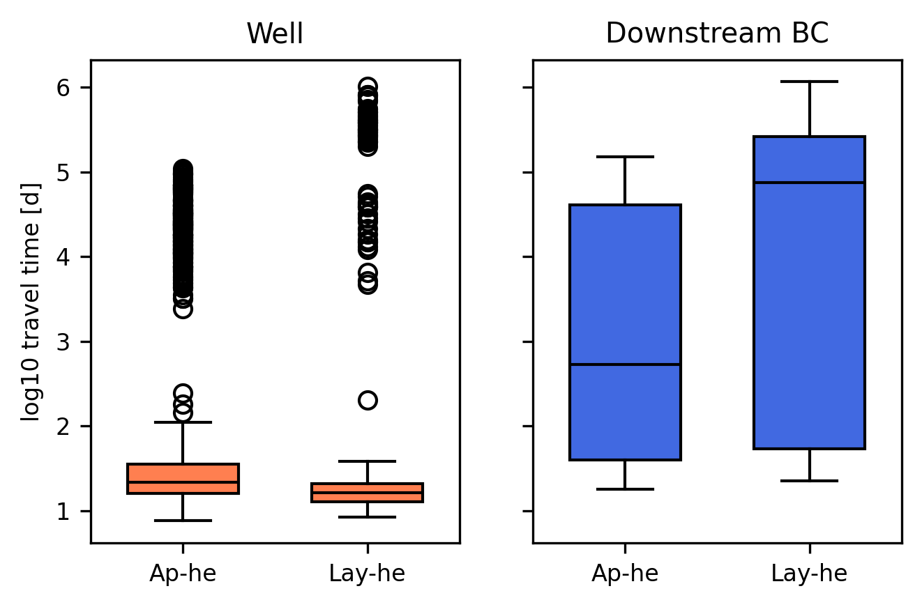
[105]:
df_plot_well = pd.DataFrame([np.log10(t_well_aphe / 86400), np.log10(t_well_layhe / 86400)]).T
df_plot_well.columns = ["Ap-he", "Lay-he"]

df_plot_bc = pd.DataFrame([np.log10(t_bc_aphe / 86400), np.log10(t_bc_layhe / 86400)]).T
df_plot_bc.columns = ["Ap-he", "Lay-he"]
[106]:
fig, ax= plt.subplots(1, 2, figsize=(5, 3), dpi=300, sharey=True)

axi = ax[0]
positions = [0, 1]
df_plot_well.plot.box(positions=positions, ax=axi, patch_artist=True, showfliers=True, widths=0.6,
                boxprops=dict(facecolor="coral"),
                whiskerprops=dict(color="black"),
                medianprops=dict(color="black"),
                capprops=dict(color="black"))
axi.set_ylabel("log10 travel time [d]")
axi.set_title("Well")

axi = ax[1]
positions = [0, 1]
df_plot_bc.plot.box(positions=positions, ax=axi, patch_artist=True, showfliers=True, widths=0.6,
                boxprops=dict(facecolor="royalblue"),
                whiskerprops=dict(color="black"),
                medianprops=dict(color="black"),
                capprops=dict(color="black"))

axi.set_title("Downstream BC")
[106]:
Text(0.5, 1.0, 'Downstream BC')
[107]:
import ArchPy.ap_mf
[108]:
np.random.seed(1312)
for i in range(10):
    ip = np.random.randint(2000)
    df_p = archpy_flow.prt_get_facies_path_particle(ip)
    ArchPy.ap_mf.plot_particle_facies_sequence(T1, df=df_p, plot_distance=True, proportions=False, plot_time=False)


[109]:
df_all = archpy_flow.prt_get_pathlines()
df = df_all.loc[df_all.irpt==1639]
df
[109]:
| irpt | icell | kper | kstp | imdl | iprp | ilay | izone | istatus | ireason | trelease | t | x | y | z | name | |
|---|---|---|---|---|---|---|---|---|---|---|---|---|---|---|---|---|
| 207133 | 1639 | 112011 | 1 | 1 | 1 | 1 | 23 | 0 | 1 | 0 | 0.0 | 0.000000e+00 | 15.032296 | 43.731413 | -10.856335 | NaN |
| 207134 | 1639 | 112011 | 1 | 1 | 1 | 1 | 23 | 0 | 1 | 1 | 0.0 | 6.952132e+03 | 15.272026 | 43.896049 | -10.800000 | NaN |
| 207135 | 1639 | 107011 | 1 | 1 | 1 | 1 | 22 | 0 | 1 | 1 | 0.0 | 2.720498e+04 | 15.999072 | 44.405281 | -10.650000 | NaN |
| 207136 | 1639 | 102011 | 1 | 1 | 1 | 1 | 21 | 0 | 1 | 1 | 0.0 | 4.060122e+04 | 16.500000 | 44.755302 | -10.560089 | NaN |
| 207137 | 1639 | 102012 | 1 | 1 | 1 | 1 | 21 | 0 | 1 | 1 | 0.0 | 5.125454e+04 | 16.901001 | 45.000000 | -10.535387 | NaN |
| ... | ... | ... | ... | ... | ... | ... | ... | ... | ... | ... | ... | ... | ... | ... | ... | ... |
| 207204 | 1639 | 92540 | 1 | 1 | 1 | 1 | 19 | 0 | 1 | 1 | 0.0 | 1.414964e+06 | 60.000000 | 36.949094 | -10.257452 | NaN |
| 207205 | 1639 | 92541 | 1 | 1 | 1 | 1 | 19 | 0 | 1 | 1 | 0.0 | 1.415138e+06 | 60.056596 | 36.931343 | -10.350000 | NaN |
| 207206 | 1639 | 97541 | 1 | 1 | 1 | 1 | 20 | 0 | 1 | 1 | 0.0 | 1.415367e+06 | 60.135468 | 36.906269 | -10.500000 | NaN |
| 207207 | 1639 | 102541 | 1 | 1 | 1 | 1 | 21 | 0 | 1 | 1 | 0.0 | 1.415547e+06 | 60.200841 | 36.885159 | -10.650000 | NaN |
| 207208 | 1639 | 107541 | 1 | 1 | 1 | 1 | 22 | 0 | 5 | 3 | 0.0 | 1.415547e+06 | 60.200841 | 36.885159 | -10.650000 | NaN |
76 rows × 16 columns
[110]:
np.random.seed(15)
[111]:
n = 2000
xp = np.random.uniform(125, 149, n)
yp = np.random.uniform(T1.yg[-1]*0.2 + T1.yg[0], T1.yg[-1]*0.8, n)
zp = np.random.uniform(-9, -11, n)
list_p_coords = []
for i in range(n):
    list_p_coords.append((xp[i], yp[i], zp[i]))
plt.scatter(xp, yp, c="red", s=3)
gwf.modelgrid.plot(alpha=.1)
[111]:
<matplotlib.collections.LineCollection at 0x1d5d1a174d0>
[112]:
archpy_flow.prt_create(prt_name="test_prt", workspace="ws_prt", trackdir="backward", list_p_coords=list_p_coords)
archpy_flow.set_porosity(prop_key="Porosity", iu=0, ifa=0, ip=0)
archpy_flow.prt_run(silent=False)
c:\Users\schorppl\.conda\envs\archpy_work\Lib\site-packages\flopy\utils\gridintersect.py:123: DeprecationWarning: Note `method="structured"` is deprecated. Pass `method="vertex"` to silence this warning. This will be the new default in a future release and this keyword argument will be removed.
  warnings.warn(
writing simulation...
  writing simulation name file...
  writing simulation tdis package...
  writing solution package ems...
  writing model test_prt...
    writing model name file...
    writing package mip...
    writing package dis...
    writing package prp...
    writing package oc...
    writing package fmi...
FloPy is using the following executable to run the model: \\home\schorppl$\exe\mf6.exe
                                   MODFLOW 6
                U.S. GEOLOGICAL SURVEY MODULAR HYDROLOGIC MODEL
                            VERSION 6.6.1 02/10/2025

   MODFLOW 6 compiled Feb 14 2025 13:40:10 with Intel(R) Fortran Intel(R) 64
   Compiler Classic for applications running on Intel(R) 64, Version 2021.7.0
                             Build 20220726_000000

This software has been approved for release by the U.S. Geological
Survey (USGS). Although the software has been subjected to rigorous
review, the USGS reserves the right to update the software as needed
pursuant to further analysis and review. No warranty, expressed or
implied, is made by the USGS or the U.S. Government as to the
functionality of the software and related material nor shall the
fact of release constitute any such warranty. Furthermore, the
software is released on condition that neither the USGS nor the U.S.
Government shall be held liable for any damages resulting from its
authorized or unauthorized use. Also refer to the USGS Water
Resources Software User Rights Notice for complete use, copyright,
and distribution information.


 MODFLOW runs in SEQUENTIAL mode

 Run start date and time (yyyy/mm/dd hh:mm:ss): 2025/10/06 14:11:04

 Writing simulation list file: mfsim.lst
 Using Simulation name file: mfsim.nam

    Solving:  Stress period:     1    Time step:     1

 Run end date and time (yyyy/mm/dd hh:mm:ss): 2025/10/06 14:11:07
 Elapsed run time:  3.476 Seconds

 Normal termination of simulation.
[113]:
df_all = archpy_flow.prt_get_pathlines()
[114]:
plt.figure(figsize=(5, 2), dpi=300)

# gwf.modelgrid.plot(alpha=.1)
for i in range(1, 2000):
    path = df_all.loc[df_all.irpt == i]
    plt.plot(path["x"], path["y"], linewidth=.1, color="royalblue")

plt.xlabel("X [m]")
plt.ylabel("Y [m]")
[114]:
Text(0, 0.5, 'Y [m]')
[115]:
self = archpy_flow
[116]:
sim_dir = self.sim_prt.sim_path
csv_name = self.sim_prt.prt[0].oc.trackcsv_filerecord.array[0][0]
csv_path = os.path.join(sim_dir, csv_name)
df = pd.read_csv(csv_path)
df = df.loc[df.irpt==9]
[117]:
time_ordered = df["t"].values.copy()
time_ordered *= 1/86400
dt = np.diff(time_ordered)

# add a column to track distance traveled
distances = ((df[["x", "y", "z"]].iloc[1:].values - df[["x", "y", "z"]].iloc[:-1].values)**2).sum(1)**0.5

# store everything in a new dataframe
df_all = pd.DataFrame(columns=["dt", "time", "distance", "cum_distance", "x", "y", "z"])
df_all["dt"] = dt
df_all["time"] = time_ordered[1:]
df_all["distance"] = distances
df_all["cum_distance"] = df_all["distance"].cumsum()
df_all["x"] = df["x"].values[1:]
df_all["y"] = df["y"].values[1:]
df_all["z"] = df["z"].values[1:]
[118]:
nx = self.get_gwf().modelgrid.ncol
ny = self.get_gwf().modelgrid.nrow
cells_path = ArchPy.ap_mf.get_locs(df.icell-1, nx, ny)
cells_path = np.array(cells_path)[1:]

# check that no cells path exceed the grid
cells_path[:, 0][cells_path[:, 0] >= self.T1.nz] = self.T1.nz - 1
cells_path[:, 1][cells_path[:, 1] >= self.T1.ny] = self.T1.ny - 1
cells_path[:, 2][cells_path[:, 2] >= self.T1.nx] = self.T1.nx - 1
[119]:
facies = self.T1.get_facies(0, 0, all_data=False)
facies = np.flip(np.flipud(facies), axis=1)
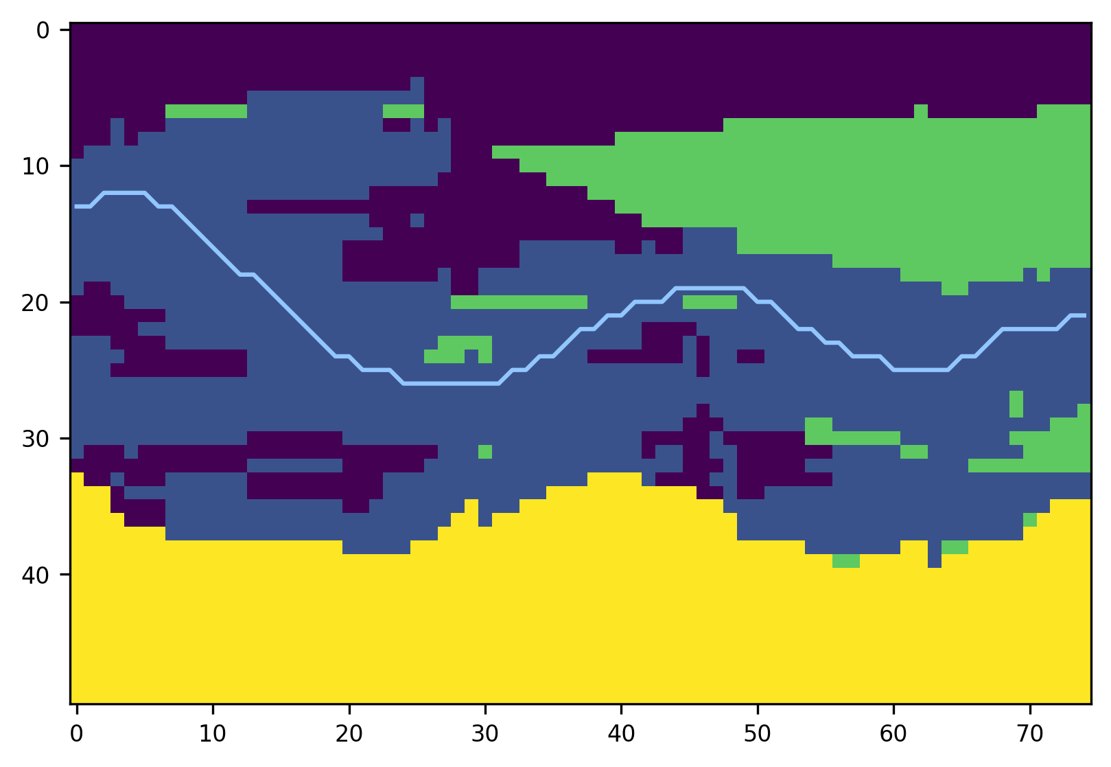
[120]:
plt.figure(dpi=300)
plt.imshow(facies[:, cells_path[:, 1], cells_path[:, 2]], vmin=1, vmax=5)
plt.plot(cells_path[:, 0])
[120]:
[<matplotlib.lines.Line2D at 0x1d5d7a4fa40>]
NR-heterogeneous mode
[215]:
archpy_flow = archpy2modflow(T1, exe_name=mf6_exe_path, model_dir="new_res_hetero")  # create the modflow model
archpy_flow.create_sim(grid_mode="new_resolution", iu=0, unit_limit=None, factor_x=4, factor_y=2, factor_z=2)  # create the simulation object and choose a certain discretization
archpy_flow.set_k("K", iu=0, ifa=0, ip=0, log=True)  # set the hydraulic conductivity
Simulation created with the following parameters:
Grid mode: new_resolution
To retrieve the simulation, use the get_sim() method
[216]:
from ArchPy.uppy import upscale_k, rotate_point

self = archpy_flow
prop_key = "K"
iu = 0
ifa = 0
ip = 0
log = True
from ArchPy.uppy import upscale_k


prop = self.T1.get_prop(prop_key)[iu, ifa, ip]
prop = np.flip(np.flipud(prop), axis=1)  # flip the array to have the same orientation as the ArchPy table
if log:
    prop = 10**prop
new_prop, _, _ = upscale_k(prop, method="simplified_renormalization",
                        dx=self.T1.get_sx(), dy=self.T1.get_sy(), dz=self.T1.get_sz(),
                        factor_x=self.factor_x, factor_y=self.factor_y, factor_z=self.factor_z)

# fill nan values
# new_prop[np.isnan(new_prop)] = np.nanmean(new_prop)
[217]:
new_prop
[217]:
array([[[8.32609353e-05, 2.71230057e-04, 4.24658011e-04, ...,
         5.73240807e-04, 6.93446533e-04, 1.29933221e-03],
        [1.44450787e-04, 4.17324564e-04, 4.96956819e-04, ...,
         2.33076627e-04, 3.97862842e-04, 9.86264710e-04],
        [2.31615460e-04, 6.19503471e-04, 6.75846878e-04, ...,
         1.12077139e-04, 2.53304313e-04, 6.24695883e-04],
        ...,
        [3.94693125e-04, 2.29263461e-04, 7.92197847e-05, ...,
         1.33543271e-03, 7.16278293e-04, 1.71205073e-04],
        [3.58655216e-04, 4.03808104e-04, 1.47935676e-04, ...,
         1.85078066e-03, 1.18666428e-03, 1.91316906e-04],
        [2.58671573e-04, 5.56179840e-04, 4.42109625e-04, ...,
         2.20347060e-03, 1.13817022e-03, 1.75655270e-04]],

       [[7.48763759e-05, 2.40885570e-04, 4.25562931e-04, ...,
         5.67331673e-04, 6.67760724e-04, 1.19102848e-03],
        [7.56787934e-05, 2.58930989e-04, 3.41639996e-04, ...,
         2.32346654e-04, 3.59904216e-04, 8.96483010e-04],
        [5.15365293e-05, 2.92249399e-04, 4.56086990e-04, ...,
         1.07608056e-04, 2.36007051e-04, 5.77659521e-04],
        ...,
        [3.93422580e-04, 2.26449452e-04, 7.97391096e-05, ...,
         1.30951916e-03, 6.75105178e-04, 1.60346926e-04],
        [3.41865182e-04, 4.11197406e-04, 1.53806085e-04, ...,
         1.85281827e-03, 1.07370879e-03, 1.70131713e-04],
        [2.34228342e-04, 5.69383638e-04, 4.69705525e-04, ...,
         2.18568049e-03, 1.01781501e-03, 1.43632552e-04]],

       [[6.22142624e-09, 6.99853796e-09, 4.29686025e-09, ...,
         2.79137575e-04, 4.64879107e-04, 9.52326768e-04],
        [9.65605083e-09, 9.86897010e-09, 9.18672805e-09, ...,
         1.48180505e-04, 3.46547740e-04, 8.15381202e-04],
        [9.77428928e-09, 1.23959792e-08, 1.81857968e-08, ...,
         9.04396727e-05, 2.24142631e-04, 5.40536031e-04],
        ...,
        [3.94948836e-04, 2.33148189e-04, 8.22526449e-05, ...,
         1.27297932e-03, 6.51007706e-04, 1.56749575e-04],
        [3.52479485e-04, 4.32536801e-04, 1.64275409e-04, ...,
         1.85996553e-03, 1.04886865e-03, 1.62576354e-04],
        [2.36256169e-04, 5.83373884e-04, 4.92656769e-04, ...,
         2.14994902e-03, 1.00024337e-03, 1.36181796e-04]],

       ...,

       [[1.00000001e-10, 1.00000001e-10, 1.29424956e-10, ...,
         1.00000001e-10, 1.00000001e-10, 1.00000001e-10],
        [1.00000001e-10, 1.00000001e-10, 2.33889149e-05, ...,
         1.00000001e-10, 1.00000001e-10, 1.00000001e-10],
        [1.00000001e-10, 1.00000001e-10, 3.70463823e-10, ...,
         1.00000001e-10, 1.00000001e-10, 1.00000001e-10],
        ...,
        [1.00000001e-10, 1.00000001e-10, 1.00000001e-10, ...,
         1.00000001e-10, 1.00000001e-10, 1.00000001e-10],
        [1.00000001e-10, 1.00000001e-10, 1.00000001e-10, ...,
         1.00000001e-10, 1.00000001e-10, 1.00000001e-10],
        [1.00000001e-10, 1.00000001e-10, 1.00000001e-10, ...,
         1.00000001e-10, 1.00000001e-10, 1.00000001e-10]],

       [[1.00000001e-10, 1.00000001e-10, 1.00000001e-10, ...,
         1.00000001e-10, 1.00000001e-10, 1.00000001e-10],
        [1.00000001e-10, 1.00000001e-10, 1.00000001e-10, ...,
         1.00000001e-10, 1.00000001e-10, 1.00000001e-10],
        [1.00000001e-10, 1.00000001e-10, 1.00000001e-10, ...,
         1.00000001e-10, 1.00000001e-10, 1.00000001e-10],
        ...,
        [1.00000001e-10, 1.00000001e-10, 1.00000001e-10, ...,
         1.00000001e-10, 1.00000001e-10, 1.00000001e-10],
        [1.00000001e-10, 1.00000001e-10, 1.00000001e-10, ...,
         1.00000001e-10, 1.00000001e-10, 1.00000001e-10],
        [1.00000001e-10, 1.00000001e-10, 1.00000001e-10, ...,
         1.00000001e-10, 1.00000001e-10, 1.00000001e-10]]])
[202]:
sim = archpy_flow.get_sim()
gwf = archpy_flow.get_gwf()
[203]:
gwf.modelgrid.nlay * gwf.modelgrid.nrow * gwf.modelgrid.ncol
[203]:
15625
[204]:
sim.ims.remove()
inner_dvclose = 1e-5
ims = fp.mf6.ModflowIms(sim, complexity="moderate", inner_dvclose=inner_dvclose)
[205]:
# add BC at left and right on all layers
h1 = .3
h2 = 0
T_1 = 10  # temperature at left boundary
T_2 = 10  # temperature at right boundary
chd_data = []

a = np.zeros((gwf.modelgrid.nlay, gwf.modelgrid.nrow, gwf.modelgrid.ncol), dtype=bool)
a[:, :, 0] = 1
lst_chd = array2cellids(a, gwf.dis.idomain.array)
for cellid in lst_chd:
    chd_data.append((cellid, h1, T_1))

chd1 = fp.mf6.ModflowGwfchd(gwf, stress_period_data=chd_data, save_flows=True, auxiliary="TEMPERATURE", pname="CHD-1")

chd_data = []
a = np.zeros((gwf.modelgrid.nlay, gwf.modelgrid.nrow, gwf.modelgrid.ncol), dtype=bool)
a[:, :, -1] = 1
lst_chd = array2cellids(a, gwf.dis.idomain.array)
for cellid in lst_chd:
    chd_data.append((cellid, h2, T_2))

chd2 = fp.mf6.ModflowGwfchd(gwf, stress_period_data=chd_data, save_flows=True, auxiliary="TEMPERATURE", pname="CHD-2")
[206]:
# add an injection well in the middle of the model
well_data = []
Q_well = 0.0015  # m3/s
T_well = 7  # temperature of the injected water
cellid_well = (int(21/50 *  gwf.dis.nlay.array), gwf.dis.nrow.array // 2, gwf.dis.ncol.array // 2)
well_data.append((cellid_well, Q_well, T_well))
wel = fp.mf6.ModflowGwfwel(gwf, stress_period_data=well_data, save_flows=True, auxiliary="TEMPERATURE", pname="WEL-INJ")

# production well
well_data = []
Q_well = -Q_well # m3/s
cellid_well = (int(21/50 *  gwf.dis.nlay.array), gwf.dis.nrow.array // 2, int(gwf.dis.ncol.array // 2.5))
well_data.append((cellid_well, Q_well))
wel = fp.mf6.ModflowGwfwel(gwf, stress_period_data=well_data, save_flows=True, pname="WEL-PROD")
[127]:
sim.write_simulation()
sim.run_simulation()
writing simulation...
  writing simulation name file...
  writing simulation tdis package...
  writing solution package ims_-1...
  writing model test...
    writing model name file...
    writing package dis...
    writing package ic...
    writing package oc...
    writing package npf...
    writing package chd-1...
INFORMATION: maxbound in ('gwf6', 'chd', 'dimensions') changed to 625 based on size of stress_period_data
    writing package chd-2...
INFORMATION: maxbound in ('gwf6', 'chd', 'dimensions') changed to 625 based on size of stress_period_data
    writing package wel-inj...
INFORMATION: maxbound in ('gwf6', 'wel', 'dimensions') changed to 1 based on size of stress_period_data
    writing package wel-prod...
INFORMATION: maxbound in ('gwf6', 'wel', 'dimensions') changed to 1 based on size of stress_period_data
FloPy is using the following executable to run the model: \\home\schorppl$\exe\mf6.exe
                                   MODFLOW 6
                U.S. GEOLOGICAL SURVEY MODULAR HYDROLOGIC MODEL
                            VERSION 6.6.1 02/10/2025

   MODFLOW 6 compiled Feb 14 2025 13:40:10 with Intel(R) Fortran Intel(R) 64
   Compiler Classic for applications running on Intel(R) 64, Version 2021.7.0
                             Build 20220726_000000

This software has been approved for release by the U.S. Geological
Survey (USGS). Although the software has been subjected to rigorous
review, the USGS reserves the right to update the software as needed
pursuant to further analysis and review. No warranty, expressed or
implied, is made by the USGS or the U.S. Government as to the
functionality of the software and related material nor shall the
fact of release constitute any such warranty. Furthermore, the
software is released on condition that neither the USGS nor the U.S.
Government shall be held liable for any damages resulting from its
authorized or unauthorized use. Also refer to the USGS Water
Resources Software User Rights Notice for complete use, copyright,
and distribution information.


 MODFLOW runs in SEQUENTIAL mode

 Run start date and time (yyyy/mm/dd hh:mm:ss): 2025/10/06 14:11:39

 Writing simulation list file: mfsim.lst
 Using Simulation name file: mfsim.nam

    Solving:  Stress period:     1    Time step:     1

 Run end date and time (yyyy/mm/dd hh:mm:ss): 2025/10/06 14:11:40
 Elapsed run time:  0.394 Seconds

 Normal termination of simulation.
[127]:
(True, [])
[128]:
from flopy.export.vtk import Vtk

vert_exag = 3
vtk = Vtk(model=gwf, binary=False, vertical_exageration=vert_exag, smooth=True)
vtk.add_model(gwf)

heads = archpy_flow.get_heads()
vtk.add_array(heads, name="heads")
vtk.add_array(np.log10(gwf.npf.k.array), name="K")

gwf_mesh = vtk.to_pyvista()
ghosts = np.argwhere(gwf_mesh["idomain"] <= 0)
gwf_mesh.remove_cells(ghosts, inplace=True)

pl = pv.Plotter(notebook=True)
pl.add_mesh(gwf_mesh, opacity=1, show_edges=True, scalars="heads", cmap="gist_ncar", edge_opacity=0.3, clim=[0, 0.3])
# pl.show(screenshot="E:/switchdrive/Post_doc/figures/articles/archpy 2/raw/flow_NR_he.png", window_size=[1300, 900], auto_close=False)

pl.show()
[129]:
heads = archpy_flow.get_heads()
[130]:
cobj = gwf.output.budget()
qx, qy, qz = fp.utils.postprocessing.get_specific_discharge(
        cobj.get_data(text="DATA-SPDIS", kstpkper=(0, 0))[0], gwf)

# plot cross section
from flopy.plot import PlotCrossSection
fig, ax = plt.subplots(1, 1, figsize=(10, 3), dpi=300)
cross_section = PlotCrossSection(model=gwf, line={"row": 12})
# cross_section.plot_array(np.log10(gwf.npf.k.array), cmap="Blues", ax=ax)
cross_section.plot_array(heads, cmap="gist_ncar", ax=ax)
cross_section.plot_bc("CHD-1", color="red", ax=ax)
cross_section.plot_bc("CHD-2", color="blue", ax=ax)
cross_section.plot_bc("WEL-INJ", color="brown", ax=ax)
cross_section.plot_bc("WEL-PROD", color="white", ax=ax)
cross_section.plot_vector(qx, qy, qz, color="black", normalize=True, kstep=2, hstep=2, ax=ax, scale=30)
cross_section.plot_grid(linewidth=0.2, color="black")
# fig.savefig("E:/switchdrive/Post_doc/figures/articles/archpy 2/raw/flow_NR_he_cross_section.png", dpi=300, bbox_inches="tight")
plt.xlabel("X [m]")
plt.ylabel("Z [m]")
[130]:
Text(0, 0.5, 'Z [m]')
[131]:
np.random.seed(15)
[132]:
n = 2000
xp = np.random.uniform(1, 20, n)
yp = np.random.uniform(T1.yg[-1]*0.2 + T1.yg[0], T1.yg[-1]*0.8, n)
zp = np.random.uniform(-9, -11, n)
list_p_coords = []
for i in range(n):
    list_p_coords.append((xp[i], yp[i], zp[i]))
plt.scatter(xp, yp, c="red", s=3)
gwf.modelgrid.plot(alpha=.1)
[132]:
<matplotlib.collections.LineCollection at 0x1d5c5385fd0>
[133]:
archpy_flow.prt_create(prt_name="test_prt", workspace="ws_prt", trackdir="forward", list_p_coords=list_p_coords)
archpy_flow.set_porosity(prop_key="Porosity", iu=0, ifa=0, ip=0)
archpy_flow.prt_run(silent=False)
c:\Users\schorppl\.conda\envs\archpy_work\Lib\site-packages\flopy\utils\gridintersect.py:123: DeprecationWarning: Note `method="structured"` is deprecated. Pass `method="vertex"` to silence this warning. This will be the new default in a future release and this keyword argument will be removed.
  warnings.warn(
writing simulation...
  writing simulation name file...
  writing simulation tdis package...
  writing solution package ems...
  writing model test_prt...
    writing model name file...
    writing package mip...
    writing package dis...
    writing package prp...
    writing package oc...
    writing package fmi...
FloPy is using the following executable to run the model: \\home\schorppl$\exe\mf6.exe
                                   MODFLOW 6
                U.S. GEOLOGICAL SURVEY MODULAR HYDROLOGIC MODEL
                            VERSION 6.6.1 02/10/2025

   MODFLOW 6 compiled Feb 14 2025 13:40:10 with Intel(R) Fortran Intel(R) 64
   Compiler Classic for applications running on Intel(R) 64, Version 2021.7.0
                             Build 20220726_000000

This software has been approved for release by the U.S. Geological
Survey (USGS). Although the software has been subjected to rigorous
review, the USGS reserves the right to update the software as needed
pursuant to further analysis and review. No warranty, expressed or
implied, is made by the USGS or the U.S. Government as to the
functionality of the software and related material nor shall the
fact of release constitute any such warranty. Furthermore, the
software is released on condition that neither the USGS nor the U.S.
Government shall be held liable for any damages resulting from its
authorized or unauthorized use. Also refer to the USGS Water
Resources Software User Rights Notice for complete use, copyright,
and distribution information.


 MODFLOW runs in SEQUENTIAL mode

 Run start date and time (yyyy/mm/dd hh:mm:ss): 2025/10/06 14:11:44

 Writing simulation list file: mfsim.lst
 Using Simulation name file: mfsim.nam

    Solving:  Stress period:     1    Time step:     1

 Run end date and time (yyyy/mm/dd hh:mm:ss): 2025/10/06 14:11:45
 Elapsed run time:  0.886 Seconds

 Normal termination of simulation.
[134]:
df_all = archpy_flow.prt_get_pathlines()
[135]:
t_well_layhe = []
t_bc_layhe = []
for i in range(1, 2000):
    xmax = df_all.loc[df_all.irpt==i].iloc[-1].x
    if xmax < 65:
        t_well_layhe.append(df_all.loc[df_all.irpt==i].iloc[-1].t)
    else:
        t_bc_layhe.append(df_all.loc[df_all.irpt==i].iloc[-1].t)

t_well_layhe = np.array(t_well_layhe)
t_bc_layhe = np.array(t_bc_layhe)
np.save("t_well_nrhe.npy", t_well_layhe)
np.save("t_bc_nrhe.npy", t_bc_layhe)
Modflow grid mode heterogeneous
Create a refined grid
[235]:
import flopy
from flopy.utils.gridgen import Gridgen
from flopy.export.vtk import Vtk

gridgen_path = "../../../../exe/gridgen.exe"
[236]:
nlay = 10
nrow = 26
ncol = 40
Lx = 150
Ly = 75
delr = Lx / ncol
delc = Ly / nrow
top = -7.5

ox = 0
oy = 0
oz = -15
dz = (oz - top) / nlay
botm = np.linspace(top + dz, oz, nlay)

sim = flopy.mf6.MFSimulation(
    sim_name="asdf", sim_ws="ws", exe_name="mf6")
tdis = flopy.mf6.ModflowTdis(sim, time_units="DAYS", perioddata=[[1.0, 1, 1.0]])
ms = flopy.mf6.ModflowGwf(sim, modelname="asdf", save_flows=True)
dis = flopy.mf6.ModflowGwfdis(
    ms,
    nlay=nlay,
    nrow=nrow,
    ncol=ncol,
    delr=delr,
    delc=delc,
    top=top,
    botm=botm,
    xorigin=0,  # gridgen will be applied on a grid with origin at 0, 0
    yorigin=0,
)

# create Gridgen object
g = Gridgen(ms.modelgrid, model_ws="gridgen_ws", exe_name=gridgen_path)

well1_coord = (T1.xg[T1.nx // 2], T1.yg[T1.ny // 2])
well2_coord = (T1.xg[int(T1.nx // 2.5)], T1.yg[T1.ny // 2])
points = [well1_coord, well2_coord]
g.add_refinement_features(points, "point", 3, range(nlay))
refshp0 = "gridgen_ws/" + "rf0"

polygon = [
    [
        (50, 30),
        (50, 45),
        (80, 45),
        (80, 30),
        (50, 30),
    ]
]
polygon = np.array(polygon)
g.add_refinement_features([polygon], "polygon", 1, range(nlay))
[237]:
g.build(verbose=False)
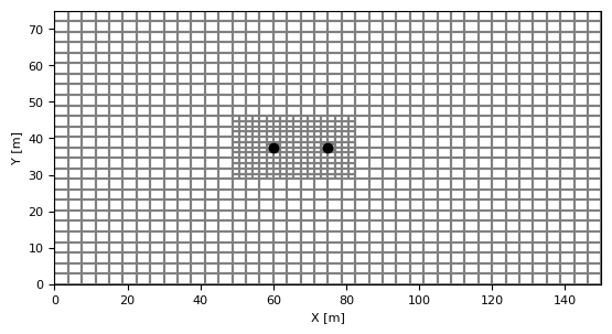
[238]:
%matplotlib inline

ms.dis.remove()
disv_gridprops = g.get_gridprops_disv()
disv = flopy.mf6.ModflowGwfdisv(ms, **disv_gridprops, xorigin=ox, yorigin=oy, angrot=0)  # create grid this time with the origin at ox, oy
# disu = flopy.mf6.ModflowGwfdisu(ms, **g.get_gridprops_disu6(), xorigin=ox, yorigin=oy, angrot=0)  # create grid this time with the origin at ox, oy

grid = ms.modelgrid
grid.plot(alpha=1, zorder=0)

plt.scatter(T1.xg[T1.nx // 2], T1.yg[T1.ny // 2], zorder=1, color="k")
plt.scatter(T1.xg[int(T1.nx // 2.5)], T1.yg[T1.ny // 2], zorder=1, color="k")

plt.ylabel("Y [m]")
plt.xlabel("X [m]")
# plt.ylim(0, 220)
# plt.xlim(-100, 220)
[238]:
Text(0.5, 0, 'X [m]')
[239]:
plt.close()
[295]:
grid.nlay * grid.ncpl
[295]:
12500
[321]:
import ArchPy.ap_mf
[322]:
archpy_flow = archpy2modflow(T1, exe_name=mf6_exe_path, model_dir="modflow_grid_hetero")  # create the modflow model
archpy_flow.create_sim(grid_mode="disv", iu=0, unit_limit=None, modflowgrid_props=g.get_gridprops_disv())  # create the simulation object and choose a certain discretization
Simulation created with the following parameters:
Grid mode: disv
To retrieve the simulation, use the get_sim() method
[323]:
archpy_flow.set_k("K", iu=0, ifa=0, ip=0, log=True, xt3doptions=None, average_facies=False) # set the hydraulic conductivity
[324]:
from ArchPy.uppy import upscale_k, rotate_point

prop_key = "K"
iu = 0
ifa = 0
ip = 0
log = True

self = archpy_flow
dx, dy, dz = self.T1.get_sx(), self.T1.get_sy(), self.T1.get_sz()
ox, oy, oz = self.T1.get_ox(), self.T1.get_oy(), self.T1.get_oz()

prop = self.T1.get_prop(prop_key)[iu, ifa, ip]
prop = np.flip(np.flipud(prop), axis=1)  # flip the array to have the same orientation as the ArchPy table
if log:
    prop = 10**prop

# get the grid object --> needs to be rotated
import copy
grid = self.get_gwf().modelgrid
grid = copy.deepcopy(grid)  # create a copy of the grid to avoid modifying the original one

# rotate grid around the origin of archpy model

# retrieve origin of the new grid and archpy grid as well as the rotation angle
xorigin, yorigin = grid.xoffset, grid.yoffset
ox_grid, oy_grid = self.T1.get_ox(), self.T1.get_oy()
angrot = self.T1.get_rot_angle()
xorigin_rot, yorigin_rot = rotate_point((xorigin, yorigin), origin=(ox_grid, oy_grid), angle=-angrot)

# rotation
grid.set_coord_info(xoff=xorigin_rot, yoff=yorigin_rot, angrot=-angrot)

# upscale
new_prop, _, _ = upscale_k(prop, method="simplified_renormalization",
                        dx=dx, dy=dy, dz=dz, ox=ox, oy=oy, oz=oz,
                        factor_x=self.factor_x, factor_y=self.factor_y, factor_z=self.factor_z,
                        grid=grid)
[325]:
new_prop
[325]:
array([[3.98672307e-05, 8.22338251e-05, 1.72688092e-04, ...,
        1.32653138e-03, 3.75687437e-04, 1.15189312e-04],
       [6.10583493e-09, 5.54328232e-09, 7.70320178e-09, ...,
        1.22436430e-03, 3.29869742e-04, 9.84170149e-05],
       [5.29816650e-09, 1.72517872e-08, 3.46159653e-03, ...,
        6.48656473e-04, 1.83651249e-04, 5.49448734e-05],
       ...,
       [1.00000001e-10, 2.61000687e-10, 3.96177158e-03, ...,
        1.00000001e-10, 1.00000001e-10, 2.81229256e-10],
       [1.00000001e-10, 1.00000001e-10, 1.61256148e-10, ...,
        1.00000001e-10, 1.00000001e-10, 1.00000001e-10],
       [1.00000001e-10, 1.00000001e-10, 1.00000001e-10, ...,
        1.00000001e-10, 1.00000001e-10, 1.00000001e-10]])
[326]:
sim = archpy_flow.get_sim()
gwf = archpy_flow.get_gwf()
[327]:
from shapely.geometry import LineString

p = np.array([(0, 0), (0, 75),
 (150, 0),
 (150, 75)])

l1 = LineString([p[0], p[1]])
l2 = LineString([p[2], p[3]])

ix = fp.utils.gridintersect.GridIntersect(mfgrid=grid)

cid1 = ix.intersects(l1).cellids
cid2 = ix.intersects(l2).cellids
h1 = 0.3
h2 = 0

# create the bc (chd package on each layers)
chd_lst = []
for ilay in range(nlay):
    chd_lst += [((ilay, id1), h1) for id1 in cid1]
for ilay in range(nlay):
    chd_lst += [((ilay, id2), h2) for id2 in cid2]

chd = fp.mf6.ModflowGwfchd(gwf, stress_period_data=chd_lst, save_flows=True, pname="CHD")
[328]:
well1_coord = (T1.xg[T1.nx // 2], T1.yg[T1.ny // 2], T1.zg[50-21])
well2_coord = (T1.xg[int(T1.nx // 2.5)], T1.yg[T1.ny // 2], T1.zg[50-21])

# add an injection well in the middle of the model
well_data = []
Q_well = 0.0015  # m3/s
T_well = 7  # temperature of the injected water
cellid_well = gwf.modelgrid.intersect(*well1_coord)
well_data.append((cellid_well, Q_well, T_well))
wel = fp.mf6.ModflowGwfwel(gwf, stress_period_data=well_data, save_flows=True, auxiliary="TEMPERATURE", pname="WEL-INJ")

# production well
well_data = []
Q_well = -Q_well # m3/s
cellid_well = gwf.modelgrid.intersect(*well2_coord)
well_data.append((cellid_well, Q_well))
wel = fp.mf6.ModflowGwfwel(gwf, stress_period_data=well_data, save_flows=True, pname="WEL-PROD")
[329]:
gwf.ic.strt.set_data(0.15)
[330]:
sim.ims.remove()
inner_dvclose = 1e-5
ims = fp.mf6.ModflowIms(sim, complexity="moderate", inner_dvclose=inner_dvclose)
[331]:
sim.write_simulation()
sim.run_simulation()
writing simulation...
  writing simulation name file...
  writing simulation tdis package...
  writing solution package ims_-1...
  writing model test...
    writing model name file...
    writing package disv...
    writing package ic...
    writing package oc...
    writing package npf...
    writing package chd...
INFORMATION: maxbound in ('gwf6', 'chd', 'dimensions') changed to 520 based on size of stress_period_data
    writing package wel-inj...
INFORMATION: maxbound in ('gwf6', 'wel', 'dimensions') changed to 1 based on size of stress_period_data
    writing package wel-prod...
INFORMATION: maxbound in ('gwf6', 'wel', 'dimensions') changed to 1 based on size of stress_period_data
FloPy is using the following executable to run the model: \\home\schorppl$\exe\mf6.exe
                                   MODFLOW 6
                U.S. GEOLOGICAL SURVEY MODULAR HYDROLOGIC MODEL
                            VERSION 6.6.1 02/10/2025

   MODFLOW 6 compiled Feb 14 2025 13:40:10 with Intel(R) Fortran Intel(R) 64
   Compiler Classic for applications running on Intel(R) 64, Version 2021.7.0
                             Build 20220726_000000

This software has been approved for release by the U.S. Geological
Survey (USGS). Although the software has been subjected to rigorous
review, the USGS reserves the right to update the software as needed
pursuant to further analysis and review. No warranty, expressed or
implied, is made by the USGS or the U.S. Government as to the
functionality of the software and related material nor shall the
fact of release constitute any such warranty. Furthermore, the
software is released on condition that neither the USGS nor the U.S.
Government shall be held liable for any damages resulting from its
authorized or unauthorized use. Also refer to the USGS Water
Resources Software User Rights Notice for complete use, copyright,
and distribution information.


 MODFLOW runs in SEQUENTIAL mode

 Run start date and time (yyyy/mm/dd hh:mm:ss): 2025/10/06 15:08:35

 Writing simulation list file: mfsim.lst
 Using Simulation name file: mfsim.nam

    Solving:  Stress period:     1    Time step:     1

 Run end date and time (yyyy/mm/dd hh:mm:ss): 2025/10/06 15:08:35
 Elapsed run time:  0.405 Seconds

 Normal termination of simulation.
[331]:
(True, [])
[332]:
from flopy.export.vtk import Vtk

vert_exag = 3
vtk = Vtk(model=gwf, binary=False, vertical_exageration=vert_exag, smooth=True)
vtk.add_model(gwf)

heads = archpy_flow.get_heads()
vtk.add_array(heads, name="heads")
vtk.add_array(np.log10(gwf.npf.k.array), name="K")

gwf_mesh = vtk.to_pyvista()

pl = pv.Plotter(notebook=True)

pl.add_mesh(gwf_mesh, opacity=1, show_edges=True, scalars="heads", cmap="gist_ncar", edge_opacity=0.3, clim=[0, 0.3])
# pl.show(screenshot="E:/switchdrive/Post_doc/figures/articles/archpy 2/raw/flow_mg_he.png", window_size=[1300, 900], auto_close=False)

pl.show()

[333]:
heads = archpy_flow.get_heads()
[334]:
plt.close()
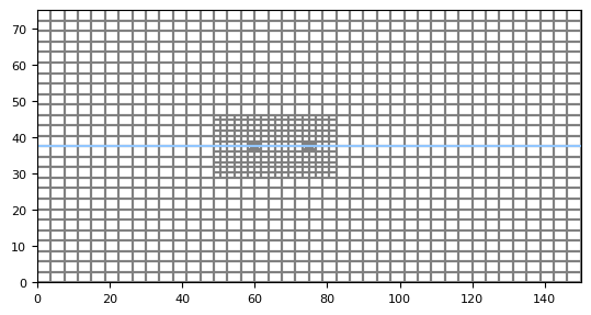
[335]:
grid.plot()
plt.plot((0, 150), (37.5, 37.5))
[335]:
[<matplotlib.lines.Line2D at 0x1d5a51ec9b0>]
[347]:
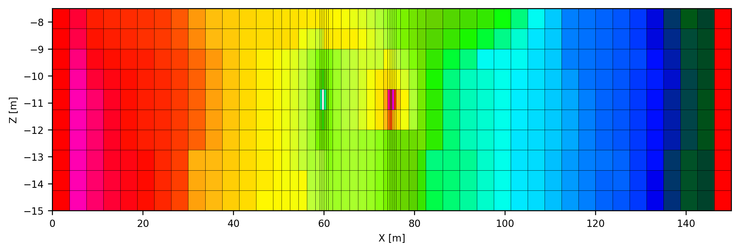
%matplotlib inline
cobj = gwf.output.budget()
qx, qy, qz = fp.utils.postprocessing.get_specific_discharge(
        cobj.get_data(text="DATA-SPDIS", kstpkper=(0, 0))[0], gwf)

# plot cross section
from flopy.plot import PlotCrossSection
fig, ax = plt.subplots(1, 1, figsize=(10, 3), dpi=300)
cross_section = PlotCrossSection(model=gwf, line={"line": ((0, 37.5), (150, 37.5))})
# cross_section.plot_array(np.log10(gwf.npf.k.array), cmap="Blues", ax=ax)
g = cross_section.plot_array(heads, cmap="gist_ncar", ax=ax)
# plt.colorbar(g)
cross_section.plot_bc("CHD", color="red", ax=ax)
# cross_section.plot_bc("CHD-2", color="blue", ax=ax)
cross_section.plot_bc("WEL-INJ", color="brown", ax=ax)
cross_section.plot_bc("WEL-PROD", color="white", ax=ax)
# cross_section.plot_vector(qx, qy, qz, color="black", normalize=True, kstep=2, hstep=2, ax=ax, scale=30)
cross_section.plot_grid(linewidth=0.2, color="black")

plt.xlabel("X [m]")
plt.ylabel("Z [m]")
# fig.savefig("E:/switchdrive/Post_doc/figures/articles/archpy 2/raw/flow_mg_he_cross_section.png", dpi=300, bbox_inches="tight")
# fig.savefig("../../../figures/articles/archpy 2/raw/archpy_he_cross_section.png", dpi=300, bbox_inches="tight")
[347]:
Text(0, 0.5, 'Z [m]')
[337]:
np.random.seed(15)
[338]:
n = 2000
xp = np.random.uniform(1, 20, n)
yp = np.random.uniform(T1.yg[-1]*0.2 + T1.yg[0], T1.yg[-1]*0.8, n)
zp = np.random.uniform(-9, -11, n)
list_p_coords = []
for i in range(n):
    list_p_coords.append((xp[i], yp[i], zp[i]))
plt.scatter(xp, yp, c="red", s=3)
gwf.modelgrid.plot(alpha=.1)
[338]:
<matplotlib.collections.LineCollection at 0x1d5a5306330>
[339]:
archpy_flow.prt_create(prt_name="test_prt", workspace="ws_prt", trackdir="forward", list_p_coords=list_p_coords)
archpy_flow.set_porosity(prop_key="Porosity", iu=0, ifa=0, ip=0)
[341]:
archpy_flow.prt_run(silent=False)
writing simulation...
  writing simulation name file...
  writing simulation tdis package...
  writing solution package ems...
  writing model test_prt...
    writing model name file...
    writing package mip...
    writing package disv...
    writing package prp...
    writing package oc...
    writing package fmi...
FloPy is using the following executable to run the model: \\home\schorppl$\exe\mf6.exe
                                   MODFLOW 6
                U.S. GEOLOGICAL SURVEY MODULAR HYDROLOGIC MODEL
                            VERSION 6.6.1 02/10/2025

   MODFLOW 6 compiled Feb 14 2025 13:40:10 with Intel(R) Fortran Intel(R) 64
   Compiler Classic for applications running on Intel(R) 64, Version 2021.7.0
                             Build 20220726_000000

This software has been approved for release by the U.S. Geological
Survey (USGS). Although the software has been subjected to rigorous
review, the USGS reserves the right to update the software as needed
pursuant to further analysis and review. No warranty, expressed or
implied, is made by the USGS or the U.S. Government as to the
functionality of the software and related material nor shall the
fact of release constitute any such warranty. Furthermore, the
software is released on condition that neither the USGS nor the U.S.
Government shall be held liable for any damages resulting from its
authorized or unauthorized use. Also refer to the USGS Water
Resources Software User Rights Notice for complete use, copyright,
and distribution information.


 MODFLOW runs in SEQUENTIAL mode

 Run start date and time (yyyy/mm/dd hh:mm:ss): 2025/10/06 15:08:51

 Writing simulation list file: mfsim.lst
 Using Simulation name file: mfsim.nam

    Solving:  Stress period:     1    Time step:     1

 Run end date and time (yyyy/mm/dd hh:mm:ss): 2025/10/06 15:08:53
 Elapsed run time:  1.408 Seconds

 Normal termination of simulation.
[342]:
df_all = archpy_flow.prt_get_pathlines()
[343]:
df_all
[343]:
| irpt | icell | kper | kstp | imdl | iprp | ilay | izone | istatus | ireason | trelease | t | x | y | z | name | |
|---|---|---|---|---|---|---|---|---|---|---|---|---|---|---|---|---|
| 0 | 1 | 4115 | 1 | 1 | 1 | 1 | 4 | 0 | 1 | 0 | 0.0 | 0.000000e+00 | 17.127536 | 48.665238 | -9.800428 | NaN |
| 1 | 1 | 4115 | 1 | 1 | 1 | 1 | 4 | 0 | 1 | 1 | 0.0 | 1.946292e+04 | 17.580640 | 49.038462 | -9.801964 | NaN |
| 2 | 1 | 4075 | 1 | 1 | 1 | 1 | 4 | 0 | 1 | 1 | 0.0 | 7.395227e+04 | 18.750000 | 49.992895 | -9.807179 | NaN |
| 3 | 1 | 4076 | 1 | 1 | 1 | 1 | 4 | 0 | 1 | 1 | 0.0 | 1.544397e+05 | 20.776522 | 51.923077 | -9.791246 | NaN |
| 4 | 1 | 4036 | 1 | 1 | 1 | 1 | 4 | 0 | 1 | 1 | 0.0 | 1.608076e+05 | 21.038229 | 52.078040 | -9.750000 | NaN |
| ... | ... | ... | ... | ... | ... | ... | ... | ... | ... | ... | ... | ... | ... | ... | ... | ... |
| 86266 | 2000 | 4404 | 1 | 1 | 1 | 1 | 4 | 0 | 1 | 1 | 0.0 | 1.835883e+06 | 59.811539 | 36.418269 | -10.252202 | NaN |
| 86267 | 2000 | 4402 | 1 | 1 | 1 | 1 | 4 | 0 | 1 | 1 | 0.0 | 1.838227e+06 | 59.782036 | 37.038885 | -10.500000 | NaN |
| 86268 | 2000 | 5652 | 1 | 1 | 1 | 1 | 5 | 0 | 1 | 1 | 0.0 | 1.838288e+06 | 59.779966 | 37.139423 | -10.517396 | NaN |
| 86269 | 2000 | 5565 | 1 | 1 | 1 | 1 | 5 | 0 | 5 | 3 | 0.0 | 1.838409e+06 | 59.773957 | 37.500000 | -10.599283 | NaN |
| 86270 | 2000 | 5650 | 1 | 1 | 1 | 1 | 5 | 0 | 1 | 1 | 0.0 | 1.838409e+06 | 59.773957 | 37.500000 | -10.599283 | NaN |
86271 rows × 16 columns
[344]:
for i in range(1, 2000):
    df_i = df_all.loc[df_all.irpt==i]
    plt.plot(df_i.x, df_i.y, color="black", alpha=0.1)
[345]:
t_well_layhe = []
t_bc_layhe = []
for i in range(1, 2000):
    xmax = df_all.loc[df_all.irpt==i].iloc[-1].x
    if xmax < 65:
        t_well_layhe.append(df_all.loc[df_all.irpt==i].iloc[-1].t)
    else:
        t_bc_layhe.append(df_all.loc[df_all.irpt==i].iloc[-1].t)

t_well_layhe = np.array(t_well_layhe)
t_bc_layhe = np.array(t_bc_layhe)
np.save("t_well_mghe.npy", t_well_layhe)
np.save("t_bc_mghe.npy", t_bc_layhe)
ArchPy mode - homogeneous
Re make an archpy model but assuming each layer completely homogeneous.
[348]:
## create pile

P1 = Pile(name = "P1",seed=1)

#units covmodel
covmodelD = gcm.CovModel2D(elem=[('cubic', {'w':0.6, 'r':[30,30]})])
covmodelD1 = gcm.CovModel2D(elem=[('cubic', {'w':0.2, 'r':[30,30]})])
covmodelC = gcm.CovModel2D(elem=[('cubic', {'w':0.2, 'r':[40,40]})])
covmodelB = gcm.CovModel2D(elem=[('cubic', {'w':0.6, 'r':[30,30]})])
covmodel_er = gcm.CovModel2D(elem=[('spherical', {'w':1, 'r':[50,50]})])


#create Lithologies
dic_s_D = {"int_method" : "grf_ineq","covmodel" : covmodelD}
dic_f_D = {"f_method":"homogenous"}
D = Unit(name="D",order=1,ID = 1,color="gold",contact="onlap",surface=Surface(contact="onlap",dic_surf=dic_s_D)
         ,dic_facies=dic_f_D)

dic_s_C = {"int_method" : "grf_ineq","covmodel" : covmodelC, "mean":-8.5}
dic_f_C = {"f_method":"homogenous"}
C = Unit(name="C", order=2, ID = 2, color="blue", contact="onlap", dic_facies=dic_f_C, surface=Surface(dic_surf=dic_s_C, contact="onlap"))

dic_s_B = {"int_method" : "grf_ineq","covmodel" : covmodelB, "mean":-9.5}
dic_f_B = {"f_method":"homogenous"}
B = Unit(name="B",order=3,ID = 3,color="purple",contact="onlap",dic_facies=dic_f_B,surface=Surface(contact="onlap",dic_surf=dic_s_B))

dic_s_A = {"int_method":"grf_ineq","covmodel": covmodelB, "mean":-13}
dic_f_A = {"f_method":"homogenous"}
A = Unit(name="A",order=4, ID = 4,color="red",contact="onlap",dic_facies=dic_f_A,surface=Surface(dic_surf = dic_s_A,contact="onlap"))

#Master pile
P1.add_unit([D,C,B,A])

# covmodels for the property model
covmodelK = gcm.CovModel3D(elem=[("exponential",{"w":0.3,"r":[30,30,10]})],alpha=-20,name="K_vario")
covmodelK2 = gcm.CovModel3D(elem=[("spherical",{"w":0.1,"r":[20,20, 5]})],alpha=0,name="K_vario_2")

facies_1 = Facies(ID = 1,name="Sand",color="yellow")
facies_2 = Facies(ID = 2,name="Gravel",color="lightgreen")
facies_4 = Facies(ID = 4,name="Clay",color="blue")
facies_7 = Facies(ID = 7,name="basement",color="red")

A.add_facies([facies_7])
B.add_facies([facies_2])
D.add_facies([facies_1])
C.add_facies([facies_4])

# property model

# K
# cm_prop1 = gcm.CovModel3D(elem = [("spherical", {"w":0.5, "r":[10, 10, 10]}),
#                                   ("cubic", {"w":0.5, "r":[15, 15, 15]})])
cm_prop2 = gcm.CovModel3D(elem = [("cubic", {"w":0.25, "r":[25, 25, 25]})])

list_facies = [facies_1, facies_2, facies_4, facies_7]
means = [-4, -2.3, -8, -10]
prop_model = ArchPy.base.Prop("K",
                              facies = list_facies,
                              covmodels = [cm_prop2, cm_prop2, cm_prop2, cm_prop2],
                                means = means,
                                int_method = "homogenous",
                                vmin = -10,
                                vmax = -1
                                )

# porosity
cm_prop2 = gcm.CovModel3D(elem = [("cubic", {"w":0.001, "r":[15, 15, 15]})])

porosity = ArchPy.base.Prop("Porosity",
                            facies = list_facies,
                            covmodels = [cm_prop2, cm_prop2, cm_prop2, cm_prop2],
                            means = [0.3, 0.3, 0.1, 0.05],
                            int_method = "homogenous",
                            vmin = 0,
                            vmax = 0.4
                            )

# alh
cm_prop1 = gcm.CovModel3D(elem = [("spherical", {"w":0.01, "r":[10, 10, 10]})])
cm_prop2 = gcm.CovModel3D(elem = [("cubic", {"w":0.01, "r":[25, 25, 5]})])

long_disp = ArchPy.base.Prop("long_disp",
                            facies = list_facies,
                            covmodels = None,
                            means = [1, 2, 10, .1],
                            int_method = "homogenous",
                            vmin = 0
                            )
top = np.ones([ny,nx])*z1
bot = np.ones([ny,nx])*z0
T1 = Arch_table(name = "P1",seed=3)
T1.set_Pile_master(P1)
T1.add_grid(dimensions, spacing, origin, top=top,bot=bot)
T1.add_prop([prop_model, porosity, long_disp])
T1.compute_surf(1)
T1.compute_facies(1)
T1.compute_prop(1)
Unit D: Surface added for interpolation
Unit C: Surface added for interpolation
Unit B: Surface added for interpolation
Unit A: Surface added for interpolation
Stratigraphic unit D added ✅
Stratigraphic unit C added ✅
Stratigraphic unit B added ✅
Stratigraphic unit A added ✅
Facies basement added to unit A ✅
Facies Gravel added to unit B ✅
Facies Sand added to unit D ✅
Facies Clay added to unit C ✅
Pile sets as Pile master
## Adding Grid ##
## Grid added and is now simulation grid ##
Property K added
Property Porosity added
Property long_disp added
Boreholes not processed, fully unconditional simulations will be tempted
########## PILE P1 ##########
Pile P1: ordering units
Stratigraphic units have been sorted according to order

#### COMPUTING SURFACE OF UNIT A
A: time elapsed for computing surface 0.18151164054870605 s

#### COMPUTING SURFACE OF UNIT B
B: time elapsed for computing surface 0.035799503326416016 s

#### COMPUTING SURFACE OF UNIT C
C: time elapsed for computing surface 0.036998748779296875 s

#### COMPUTING SURFACE OF UNIT D
D: time elapsed for computing surface 0.0 s

Time elapsed for getting domains 0.006999969482421875 s
##########################


### 0.26930785179138184: Total time elapsed for computing surfaces ###

### Unit D: facies simulation with homogenous method ####
### Unit D - realization 0 ###
Time elapsed 0.0 s

### Unit C: facies simulation with homogenous method ####
### Unit C - realization 0 ###
Time elapsed 0.0 s

### Unit B: facies simulation with homogenous method ####
### Unit B - realization 0 ###
Time elapsed 0.0 s

### Unit A: facies simulation with homogenous method ####
### Unit A - realization 0 ###
Time elapsed 0.0 s

### 0.0: Total time elapsed for computing facies ###
### 1 K property models will be modeled ###
### 1 K models done
### 1 Porosity property models will be modeled ###
### 1 Porosity models done
### 1 long_disp property models will be modeled ###
### 1 long_disp models done
[349]:
T1.plot_prop("K", cmap="jet", v_ex=3)
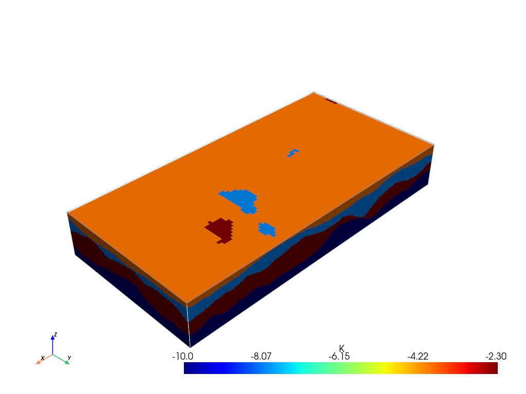
[350]:
archpy_flow = archpy2modflow(T1, exe_name=mf6_exe_path, model_dir="archpy_mode_homo")  # create the modflow model
archpy_flow.create_sim(grid_mode="archpy", iu=0, unit_limit=None)  # create the simulation object and choose a certain discretization
archpy_flow.set_k("K", iu=0, ifa=0, ip=0, log=True, average_facies=True)  # set the hydraulic conductivity
Simulation created with the following parameters:
Grid mode: archpy
To retrieve the simulation, use the get_sim() method
[351]:
sim = archpy_flow.get_sim()
gwf = archpy_flow.get_gwf()
[352]:
import flopy as fp
[353]:
sim.ims.remove()
inner_dvclose = 1e-5
ims = fp.mf6.ModflowIms(sim, complexity="moderate", inner_dvclose=inner_dvclose)
[354]:
import flopy as fp
[355]:
# add BC at left and right on all layers
h1 = .3
h2 = 0
T_1 = 10  # temperature at left boundary
T_2 = 10  # temperature at right boundary
chd_data = []

a = np.zeros((gwf.modelgrid.nlay, gwf.modelgrid.nrow, gwf.modelgrid.ncol), dtype=bool)
a[:, :, 0] = 1
lst_chd = array2cellids(a, gwf.dis.idomain.array)
for cellid in lst_chd:
    chd_data.append((cellid, h1, T_1))

chd1 = fp.mf6.ModflowGwfchd(gwf, stress_period_data=chd_data, save_flows=True, auxiliary="TEMPERATURE", pname="CHD-1")

chd_data = []
a = np.zeros((gwf.modelgrid.nlay, gwf.modelgrid.nrow, gwf.modelgrid.ncol), dtype=bool)
a[:, :, -1] = 1
lst_chd = array2cellids(a, gwf.dis.idomain.array)
for cellid in lst_chd:
    chd_data.append((cellid, h2, T_2))

chd2 = fp.mf6.ModflowGwfchd(gwf, stress_period_data=chd_data, save_flows=True, auxiliary="TEMPERATURE", pname="CHD-2")
Wells at (\(75.0, 25.0, 4.5\)) and (\(60.0, 25.0, 4.5\))
[356]:
# add an injection well in the middle of the model
well_data = []
Q_well = 0.0015  # m3/s
T_well = 7  # temperature of the injected water
cellid_well = (21, T1.ny // 2, T1.nx // 2)
well_data.append((cellid_well, Q_well, T_well))
wel = fp.mf6.ModflowGwfwel(gwf, stress_period_data=well_data, save_flows=True, auxiliary="TEMPERATURE", pname="WEL-INJ")

# production well
well_data = []
Q_well = -0.0015  # m3/s
cellid_well = (21, T1.ny // 2, int(T1.nx // 2.5))
well_data.append((cellid_well, Q_well))
wel = fp.mf6.ModflowGwfwel(gwf, stress_period_data=well_data, save_flows=True, pname="WEL-PROD")
[357]:
sim.write_simulation()
sim.run_simulation()
writing simulation...
  writing simulation name file...
  writing simulation tdis package...
  writing solution package ims_-1...
  writing model test...
    writing model name file...
    writing package dis...
    writing package ic...
    writing package oc...
    writing package npf...
    writing package chd-1...
INFORMATION: maxbound in ('gwf6', 'chd', 'dimensions') changed to 2450 based on size of stress_period_data
    writing package chd-2...
INFORMATION: maxbound in ('gwf6', 'chd', 'dimensions') changed to 2450 based on size of stress_period_data
    writing package wel-inj...
INFORMATION: maxbound in ('gwf6', 'wel', 'dimensions') changed to 1 based on size of stress_period_data
    writing package wel-prod...
INFORMATION: maxbound in ('gwf6', 'wel', 'dimensions') changed to 1 based on size of stress_period_data
FloPy is using the following executable to run the model: \\home\schorppl$\exe\mf6.exe
                                   MODFLOW 6
                U.S. GEOLOGICAL SURVEY MODULAR HYDROLOGIC MODEL
                            VERSION 6.6.1 02/10/2025

   MODFLOW 6 compiled Feb 14 2025 13:40:10 with Intel(R) Fortran Intel(R) 64
   Compiler Classic for applications running on Intel(R) 64, Version 2021.7.0
                             Build 20220726_000000

This software has been approved for release by the U.S. Geological
Survey (USGS). Although the software has been subjected to rigorous
review, the USGS reserves the right to update the software as needed
pursuant to further analysis and review. No warranty, expressed or
implied, is made by the USGS or the U.S. Government as to the
functionality of the software and related material nor shall the
fact of release constitute any such warranty. Furthermore, the
software is released on condition that neither the USGS nor the U.S.
Government shall be held liable for any damages resulting from its
authorized or unauthorized use. Also refer to the USGS Water
Resources Software User Rights Notice for complete use, copyright,
and distribution information.


 MODFLOW runs in SEQUENTIAL mode

 Run start date and time (yyyy/mm/dd hh:mm:ss): 2025/10/06 15:10:35

 Writing simulation list file: mfsim.lst
 Using Simulation name file: mfsim.nam

    Solving:  Stress period:     1    Time step:     1

 Run end date and time (yyyy/mm/dd hh:mm:ss): 2025/10/06 15:10:39
 Elapsed run time:  4.243 Seconds

 Normal termination of simulation.
[357]:
(True, [])
[358]:
from flopy.export.vtk import Vtk

vert_exag = 3
vtk = Vtk(model=gwf, binary=False, vertical_exageration=vert_exag, smooth=True)
vtk.add_model(gwf)

heads = archpy_flow.get_heads()
vtk.add_array(heads, name="heads")
vtk.add_array(np.log10(gwf.npf.k.array), name="K")

gwf_mesh = vtk.to_pyvista()
ghosts = np.argwhere(gwf_mesh["idomain"] <= 0)
gwf_mesh.remove_cells(ghosts, inplace=True)

pl = pv.Plotter(notebook=True)
# pl.add_mesh(gwf_mesh, opacity=1, show_edges=True, scalars="heads", cmap="viridis", edge_opacity=0.3, clim=[0, 0.3])

pl.add_mesh(gwf_mesh, opacity=1, show_edges=True, scalars="heads", cmap="gist_ncar", edge_opacity=0.3, clim=[0, 0.3])
# pl.show(screenshot="E:/switchdrive/Post_doc/figures/articles/archpy 2/raw/flow_archpy_ho.png", window_size=[1300, 900], auto_close=False)
pl.show()
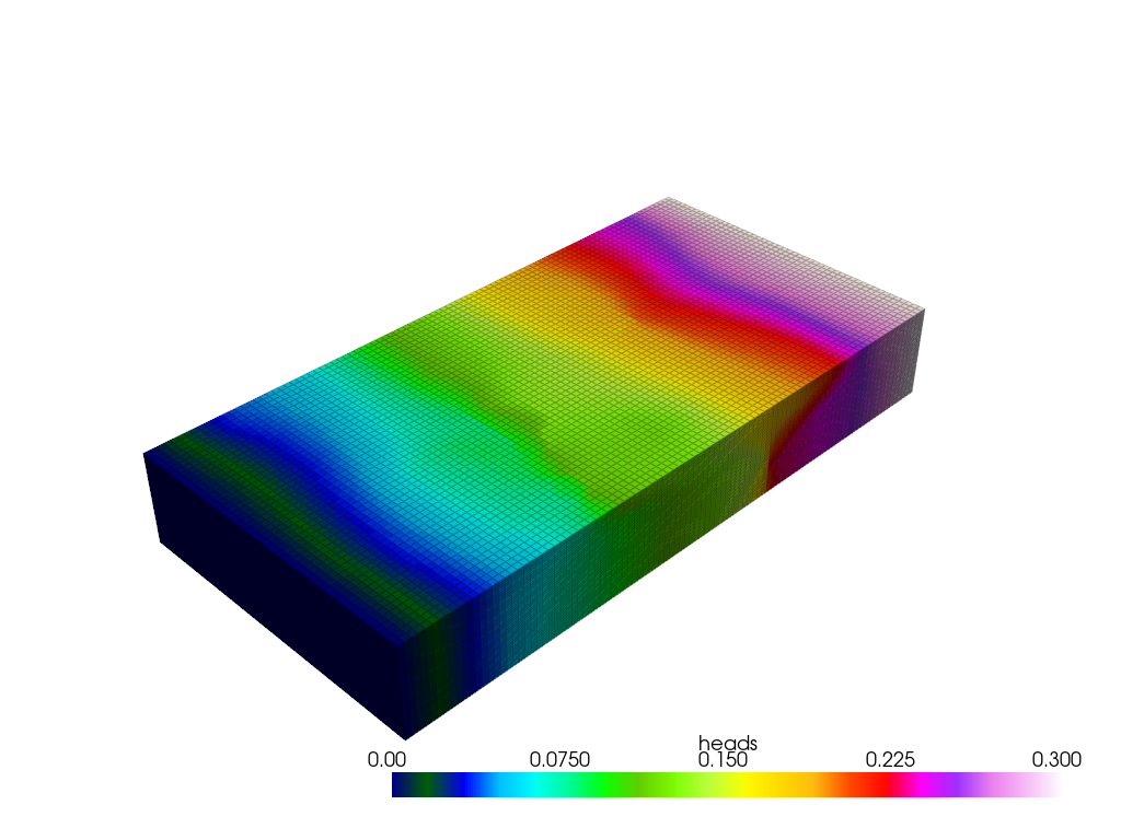
[359]:
heads = archpy_flow.get_heads()
[360]:
cobj = gwf.output.budget()
qx, qy, qz = fp.utils.postprocessing.get_specific_discharge(
        cobj.get_data(text="DATA-SPDIS", kstpkper=(0, 0))[0], gwf)

# plot cross section
from flopy.plot import PlotCrossSection
fig, ax = plt.subplots(1, 1, figsize=(10, 3), dpi=300)
cross_section = PlotCrossSection(model=gwf, line={"row": 25})
cross_section.plot_array(heads, cmap="gist_ncar", ax=ax)
cross_section.plot_bc("CHD-1", color="red", ax=ax)
cross_section.plot_bc("CHD-2", color="blue", ax=ax)
cross_section.plot_bc("WEL-INJ", color="green", ax=ax)
cross_section.plot_bc("WEL-PROD", color="orange", ax=ax)
cross_section.plot_vector(qx, qy, qz, color="black", normalize=True, kstep=4, hstep=4, ax=ax, scale=30)
cross_section.plot_grid(linewidth=0.2, color="black")

plt.xlabel("X [m]")
plt.ylabel("Z [m]")

# fig.savefig("E:/switchdrive/Post_doc/figures/articles/archpy 2/raw/flow_archpy_ho_cross_section.png", dpi=300, bbox_inches="tight")
[360]:
Text(0, 0.5, 'Z [m]')
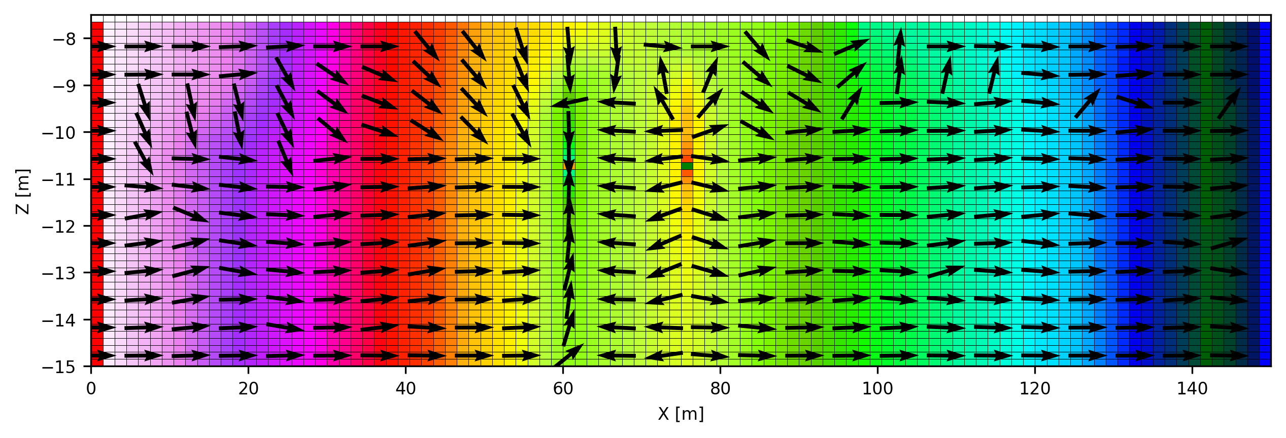
[361]:
np.random.seed(15)
[362]:
n = 2000
xp = np.random.uniform(1, 20, n)
yp = np.random.uniform(T1.yg[-1]*0.2 + T1.yg[0], T1.yg[-1]*0.8, n)
zp = np.random.uniform(-9, -11, n)
list_p_coords = []
for i in range(n):
    list_p_coords.append((xp[i], yp[i], zp[i]))
plt.scatter(xp, yp, c="red", s=3)
gwf.modelgrid.plot(alpha=.1)
[362]:
<matplotlib.collections.LineCollection at 0x1d5d76a2570>
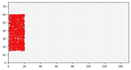
[363]:
archpy_flow.prt_create(prt_name="test_prt", workspace="ws_prt", trackdir="forward", list_p_coords=list_p_coords)
archpy_flow.set_porosity(prop_key="Porosity", iu=0, ifa=0, ip=0)
archpy_flow.prt_run(silent=False)
c:\Users\schorppl\.conda\envs\archpy_work\Lib\site-packages\flopy\utils\gridintersect.py:123: DeprecationWarning: Note `method="structured"` is deprecated. Pass `method="vertex"` to silence this warning. This will be the new default in a future release and this keyword argument will be removed.
  warnings.warn(
writing simulation...
  writing simulation name file...
  writing simulation tdis package...
  writing solution package ems...
  writing model test_prt...
    writing model name file...
    writing package mip...
    writing package dis...
    writing package prp...
    writing package oc...
    writing package fmi...
FloPy is using the following executable to run the model: \\home\schorppl$\exe\mf6.exe
                                   MODFLOW 6
                U.S. GEOLOGICAL SURVEY MODULAR HYDROLOGIC MODEL
                            VERSION 6.6.1 02/10/2025

   MODFLOW 6 compiled Feb 14 2025 13:40:10 with Intel(R) Fortran Intel(R) 64
   Compiler Classic for applications running on Intel(R) 64, Version 2021.7.0
                             Build 20220726_000000

This software has been approved for release by the U.S. Geological
Survey (USGS). Although the software has been subjected to rigorous
review, the USGS reserves the right to update the software as needed
pursuant to further analysis and review. No warranty, expressed or
implied, is made by the USGS or the U.S. Government as to the
functionality of the software and related material nor shall the
fact of release constitute any such warranty. Furthermore, the
software is released on condition that neither the USGS nor the U.S.
Government shall be held liable for any damages resulting from its
authorized or unauthorized use. Also refer to the USGS Water
Resources Software User Rights Notice for complete use, copyright,
and distribution information.


 MODFLOW runs in SEQUENTIAL mode

 Run start date and time (yyyy/mm/dd hh:mm:ss): 2025/10/06 15:10:59

 Writing simulation list file: mfsim.lst
 Using Simulation name file: mfsim.nam

    Solving:  Stress period:     1    Time step:     1

 Run end date and time (yyyy/mm/dd hh:mm:ss): 2025/10/06 15:11:02
 Elapsed run time:  2.540 Seconds

 Normal termination of simulation.
[364]:
df_all = archpy_flow.prt_get_pathlines()
[365]:
t_well_layhe = []
t_bc_layhe = []
for i in range(1, 2000):
    xmax = df_all.loc[df_all.irpt==i].iloc[-1].x
    if xmax < 65:
        t_well_layhe.append(df_all.loc[df_all.irpt==i].iloc[-1].t)
    else:
        t_bc_layhe.append(df_all.loc[df_all.irpt==i].iloc[-1].t)

t_well_layhe = np.array(t_well_layhe)
t_bc_layhe = np.array(t_bc_layhe)
np.save("t_well_apho.npy", t_well_layhe)
np.save("t_bc_apho.npy", t_bc_layhe)
[366]:
plt.hist(np.log10(t_well_layhe / 86400), density=True, alpha=.5, label="Well", color="coral", bins=30)
plt.hist(np.log10(t_bc_layhe / 86400), density=True, alpha=.5, label="Downstream BC", color="royalblue", bins=30)

plt.xlabel("log10 travel time [d]")
plt.ylabel("Density")

plt.legend()
[366]:
<matplotlib.legend.Legend at 0x1d5a51ed7c0>
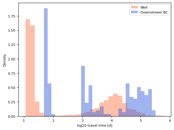
Layered homogeneous mode
[27]:
import ArchPy.ap_mf
[20]:
archpy_flow = archpy2modflow(T1, exe_name=mf6_exe_path, model_dir="layered_homo")  # create the modflow model
archpy_flow.create_sim(grid_mode="layers", iu=0, unit_limit=None, lay_sep=[1, 1, 3, 1], factor_x=2, factor_y=2, factor_z=2)  # create the simulation object and choose a certain discretization
archpy_flow.set_k("K", iu=0, ifa=0, ip=0, log=True, k_average_method="anisotropic", average_facies=True)  # set the hydraulic conductivity
Simulation created with the following parameters:
Grid mode: layers
To retrieve the simulation, use the get_sim() method
[21]:
sim = archpy_flow.get_sim()
gwf = archpy_flow.get_gwf()
[22]:
sim.ims.remove()
inner_dvclose = 1e-5
ims = fp.mf6.ModflowIms(sim, complexity="moderate", inner_dvclose=inner_dvclose)
[23]:
# add BC at left and right on all layers
h1 = .3
h2 = 0
T_1 = 10  # temperature at left boundary
T_2 = 10  # temperature at right boundary
chd_data = []

a = np.zeros((gwf.modelgrid.nlay, gwf.modelgrid.nrow, gwf.modelgrid.ncol), dtype=bool)
a[:, :, 0] = 1
lst_chd = array2cellids(a, gwf.dis.idomain.array)
for cellid in lst_chd:
    chd_data.append((cellid, h1, T_1))

chd1 = fp.mf6.ModflowGwfchd(gwf, stress_period_data=chd_data, save_flows=True, auxiliary="TEMPERATURE", pname="CHD-1")

chd_data = []
a = np.zeros((gwf.modelgrid.nlay, gwf.modelgrid.nrow, gwf.modelgrid.ncol), dtype=bool)
a[:, :, -1] = 1
lst_chd = array2cellids(a, gwf.dis.idomain.array)
for cellid in lst_chd:
    chd_data.append((cellid, h2, T_2))

chd2 = fp.mf6.ModflowGwfchd(gwf, stress_period_data=chd_data, save_flows=True, auxiliary="TEMPERATURE", pname="CHD-2")
[24]:
# add an injection well in the middle of the model
well_data = []
Q_well = 0.0015  # m3/s
T_well = 7  # temperature of the injected water
cellid_well = (2, T1.ny // 2, T1.nx // 2)
well_data.append((cellid_well, Q_well, T_well))
wel = fp.mf6.ModflowGwfwel(gwf, stress_period_data=well_data, save_flows=True, auxiliary="TEMPERATURE", pname="WEL-INJ")

# production well
well_data = []
Q_well = -Q_well # m3/s
cellid_well = (2, T1.ny // 2, int(T1.nx // 2.5))
well_data.append((cellid_well, Q_well))
wel = fp.mf6.ModflowGwfwel(gwf, stress_period_data=well_data, save_flows=True, pname="WEL-PROD")
[29]:
# update the hydraulic conductivity

k_aquifer = 5e-3
k = np.array([1e-4, 1e-8, k_aquifer, k_aquifer, k_aquifer, 1e-10])
archpy_flow.set_k(k=k, average_facies=True)
[32]:
sim.write_simulation()
sim.run_simulation()
writing simulation...
  writing simulation name file...
  writing simulation tdis package...
  writing solution package ims_-1...
  writing model test...
    writing model name file...
    writing package dis...
    writing package ic...
    writing package oc...
    writing package chd-1...
INFORMATION: maxbound in ('gwf6', 'chd', 'dimensions') changed to 300 based on size of stress_period_data
    writing package chd-2...
INFORMATION: maxbound in ('gwf6', 'chd', 'dimensions') changed to 297 based on size of stress_period_data
    writing package wel-inj...
INFORMATION: maxbound in ('gwf6', 'wel', 'dimensions') changed to 1 based on size of stress_period_data
    writing package wel-prod...
INFORMATION: maxbound in ('gwf6', 'wel', 'dimensions') changed to 1 based on size of stress_period_data
    writing package npf...
FloPy is using the following executable to run the model: \\home\schorppl$\exe\mf6.exe
                                   MODFLOW 6
                U.S. GEOLOGICAL SURVEY MODULAR HYDROLOGIC MODEL
                            VERSION 6.6.1 02/10/2025

   MODFLOW 6 compiled Feb 14 2025 13:40:10 with Intel(R) Fortran Intel(R) 64
   Compiler Classic for applications running on Intel(R) 64, Version 2021.7.0
                             Build 20220726_000000

This software has been approved for release by the U.S. Geological
Survey (USGS). Although the software has been subjected to rigorous
review, the USGS reserves the right to update the software as needed
pursuant to further analysis and review. No warranty, expressed or
implied, is made by the USGS or the U.S. Government as to the
functionality of the software and related material nor shall the
fact of release constitute any such warranty. Furthermore, the
software is released on condition that neither the USGS nor the U.S.
Government shall be held liable for any damages resulting from its
authorized or unauthorized use. Also refer to the USGS Water
Resources Software User Rights Notice for complete use, copyright,
and distribution information.


 MODFLOW runs in SEQUENTIAL mode

 Run start date and time (yyyy/mm/dd hh:mm:ss): 2025/10/06 15:22:19

 Writing simulation list file: mfsim.lst
 Using Simulation name file: mfsim.nam

    Solving:  Stress period:     1    Time step:     1

 Run end date and time (yyyy/mm/dd hh:mm:ss): 2025/10/06 15:22:19
 Elapsed run time:  0.475 Seconds

 Normal termination of simulation.
[32]:
(True, [])
[33]:
from flopy.export.vtk import Vtk

vert_exag = 3
vtk = Vtk(model=gwf, binary=False, vertical_exageration=vert_exag, smooth=True)
vtk.add_model(gwf)

heads = archpy_flow.get_heads()
vtk.add_array(heads, name="heads")
vtk.add_array(np.log10(gwf.npf.k.array), name="K")

gwf_mesh = vtk.to_pyvista()
ghosts = np.argwhere(gwf_mesh["idomain"] <= 0)
gwf_mesh.remove_cells(ghosts, inplace=True)

pl = pv.Plotter(notebook=True)
pl.add_mesh(gwf_mesh, opacity=1, show_edges=True, scalars="heads", cmap="gist_ncar", edge_opacity=0.3)
# pl.show(screenshot="../../../figures/articles/archpy 2/raw/flow_lay_ho.png", window_size=[1300, 900], auto_close=False)
# pl.show(screenshot="E:/switchdrive/Post_doc/figures/articles/archpy 2/raw/flow_lay_ho.png", window_size=[1300, 900], auto_close=False)
pl.show()
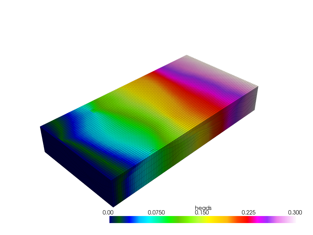
[34]:
heads = archpy_flow.get_heads()
[35]:
cobj = gwf.output.budget()
qx, qy, qz = fp.utils.postprocessing.get_specific_discharge(
        cobj.get_data(text="DATA-SPDIS", kstpkper=(0, 0))[0], gwf)

# plot cross section
from flopy.plot import PlotCrossSection
fig, ax = plt.subplots(1, 1, figsize=(10, 3), dpi=300)
cross_section = PlotCrossSection(model=gwf, line={"row": 25})
# cross_section.plot_array(np.log10(gwf.npf.k.array), cmap="Blues", ax=ax)
cont = cross_section.plot_array(heads, cmap="gist_ncar", ax=ax)
# cont = cross_section.contour_array(heads, ax=ax, levels=np.arange(0, 0.25, 0.02), linewidths=3)
# plt.clabel(cont, inline=True, fontsize=20, fmt="%.2f", colors="black")
cross_section.plot_bc("CHD-1", color="red", ax=ax)
cross_section.plot_bc("CHD-2", color="blue", ax=ax)
cross_section.plot_bc("WEL-INJ", color="brown", ax=ax)
cross_section.plot_bc("WEL-PROD", color="white", ax=ax)
cross_section.plot_vector(qx, qy, qz, color="black", normalize=True, hstep=4, kstep=1, ax=ax, scale=30)
cross_section.plot_grid(linewidth=0.5, color="black")
plt.colorbar(cont, ax=ax, label="Heads [m]", orientation="vertical", pad=0.02)
plt.xlabel("X [m]")
plt.ylabel("Z [m]")

# fig.savefig("E:/switchdrive/Post_doc/figures/articles/archpy 2/raw/flow_lay_ho_cross_section.png", dpi=300, bbox_inches="tight")
[35]:
Text(0, 0.5, 'Z [m]')
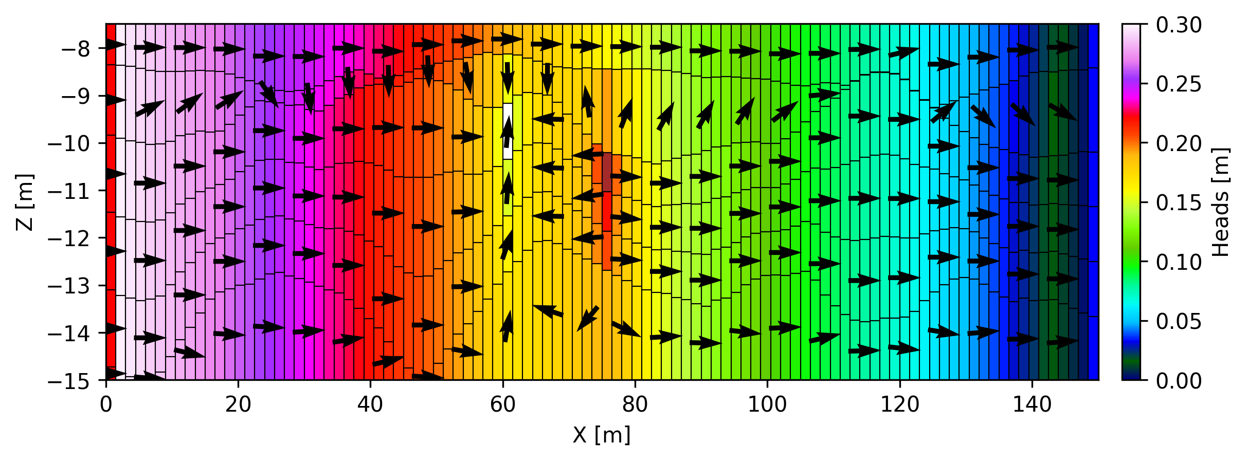
[36]:
np.random.seed(15)
[37]:
n = 2000
xp = np.random.uniform(1, 20, n)
yp = np.random.uniform(T1.yg[-1]*0.2 + T1.yg[0], T1.yg[-1]*0.8, n)
zp = np.random.uniform(-9, -11, n)
list_p_coords = []
for i in range(n):
    list_p_coords.append((xp[i], yp[i], zp[i]))
plt.scatter(xp, yp, c="red", s=3)
gwf.modelgrid.plot(alpha=.1)
[37]:
<matplotlib.collections.LineCollection at 0x21b9bf05a90>
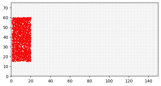
[38]:
archpy_flow.prt_create(prt_name="test_prt", workspace="ws_prt", trackdir="forward", list_p_coords=list_p_coords)
archpy_flow.set_porosity(prop_key="Porosity", iu=0, ifa=0, ip=0)
archpy_flow.prt_run(silent=False)
c:\Users\schorppl\.conda\envs\archpy_work\Lib\site-packages\flopy\utils\gridintersect.py:123: DeprecationWarning: Note `method="structured"` is deprecated. Pass `method="vertex"` to silence this warning. This will be the new default in a future release and this keyword argument will be removed.
  warnings.warn(
writing simulation...
  writing simulation name file...
  writing simulation tdis package...
  writing solution package ems...
  writing model test_prt...
    writing model name file...
    writing package mip...
    writing package dis...
    writing package prp...
    writing package oc...
    writing package fmi...
FloPy is using the following executable to run the model: \\home\schorppl$\exe\mf6.exe
                                   MODFLOW 6
                U.S. GEOLOGICAL SURVEY MODULAR HYDROLOGIC MODEL
                            VERSION 6.6.1 02/10/2025

   MODFLOW 6 compiled Feb 14 2025 13:40:10 with Intel(R) Fortran Intel(R) 64
   Compiler Classic for applications running on Intel(R) 64, Version 2021.7.0
                             Build 20220726_000000

This software has been approved for release by the U.S. Geological
Survey (USGS). Although the software has been subjected to rigorous
review, the USGS reserves the right to update the software as needed
pursuant to further analysis and review. No warranty, expressed or
implied, is made by the USGS or the U.S. Government as to the
functionality of the software and related material nor shall the
fact of release constitute any such warranty. Furthermore, the
software is released on condition that neither the USGS nor the U.S.
Government shall be held liable for any damages resulting from its
authorized or unauthorized use. Also refer to the USGS Water
Resources Software User Rights Notice for complete use, copyright,
and distribution information.


 MODFLOW runs in SEQUENTIAL mode

 Run start date and time (yyyy/mm/dd hh:mm:ss): 2025/10/06 15:22:27

 Writing simulation list file: mfsim.lst
 Using Simulation name file: mfsim.nam

    Solving:  Stress period:     1    Time step:     1

 Run end date and time (yyyy/mm/dd hh:mm:ss): 2025/10/06 15:22:29
 Elapsed run time:  1.410 Seconds

 Normal termination of simulation.
[39]:
df_all = archpy_flow.prt_get_pathlines()
[40]:
t_well_layhe = []
t_bc_layhe = []
for i in range(1, 2000):
    xmax = df_all.loc[df_all.irpt==i].iloc[-1].x
    if xmax < 65:
        t_well_layhe.append(df_all.loc[df_all.irpt==i].iloc[-1].t)
    else:
        t_bc_layhe.append(df_all.loc[df_all.irpt==i].iloc[-1].t)

t_well_layhe = np.array(t_well_layhe)
t_bc_layhe = np.array(t_bc_layhe)
np.save("t_well_layho.npy", t_well_layhe)
np.save("t_bc_layho.npy", t_bc_layhe)
[41]:
plt.hist(np.log10(t_well_layhe / 86400), density=True, alpha=.5, label="Well", color="coral", bins=30)
plt.hist(np.log10(t_bc_layhe / 86400), density=True, alpha=.5, label="Downstream BC", color="royalblue", bins=30)

plt.xlabel("log10 travel time [d]")
plt.ylabel("Density")

plt.legend()
[41]:
<matplotlib.legend.Legend at 0x21b9e0e5070>
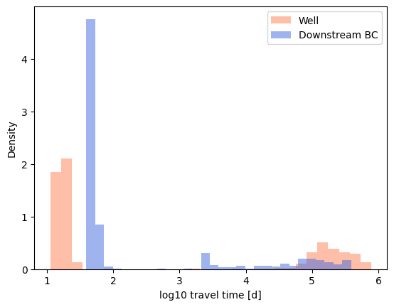
[42]:
t_well_layhe = np.load("t_well_layhe.npy")
t_bc_layhe = np.load("t_bc_layhe.npy")
t_well_aphe = np.load("t_well_aphe.npy")
t_bc_aphe = np.load("t_bc_aphe.npy")
t_well_layho = np.load("t_well_layho.npy")
t_bc_layho = np.load("t_bc_layho.npy")
t_well_apho = np.load("t_well_apho.npy")
t_bc_apho = np.load("t_bc_apho.npy")
t_well_nrhe = np.load("t_well_nrhe.npy")
t_bc_nrhe = np.load("t_bc_nrhe.npy")
t_well_mghe = np.load("t_well_mghe.npy")
t_bc_mghe = np.load("t_bc_mghe.npy")
[43]:
df_plot_well = pd.DataFrame([np.log10(t_well_aphe / 86400),np.log10(t_well_apho / 86400), np.log10(t_well_layhe / 86400), np.log10(t_well_apho / 86400), np.log10(t_well_nrhe / 86400), np.log10(t_well_mghe / 86400)]).T

df_plot_bc = pd.DataFrame([np.log10(t_bc_aphe / 86400), np.log10(t_bc_apho / 86400), np.log10(t_bc_layhe / 86400), np.log10(t_bc_layho / 86400), np.log10(t_bc_nrhe / 86400), np.log10(t_bc_mghe / 86400)]).T
df_plot_bc.columns = ["Ap-he", "Ap-ho", "Lay-he", "Lay-ho", "NR-he", "MG-he"]
df_plot_well.columns = ["Ap-he", "Ap-ho", "Lay-he", "Lay-ho", "NR-he", "MG-he"]
[44]:
import seaborn as sns
[45]:
sns.set_palette("colorblind")
[46]:
# default fontsize
matplotlib.rcParams.update({'font.size': 10})
[47]:
fig, ax= plt.subplots(1, 2, figsize=(10, 3), dpi=300, sharey=True)

axi = ax[0]
sns.violinplot(data=df_plot_well, ax=axi)
axi.set_ylabel("log10 travel time [d]")
axi.set_title("Well")

axi = ax[1]
sns.violinplot(data=df_plot_bc, ax=axi)

axi.set_title("Downstream BC")

# rotate x labels
for ax_i in ax:
    ax_i.set_xticklabels(ax_i.get_xticklabels(), rotation=45, ha="center")
    ax_i.set_xlabel("Model type")
    ax_i.grid(True)

# fig.savefig("E:/switchdrive/Post_doc/figures/articles/archpy 2/raw/travel_time_violin.png", dpi=300, bbox_inches="tight")
C:\Users\schorppl\AppData\Local\Temp\ipykernel_23664\605621732.py:15: UserWarning: set_ticklabels() should only be used with a fixed number of ticks, i.e. after set_ticks() or using a FixedLocator.
  ax_i.set_xticklabels(ax_i.get_xticklabels(), rotation=45, ha="center")
C:\Users\schorppl\AppData\Local\Temp\ipykernel_23664\605621732.py:15: UserWarning: set_ticklabels() should only be used with a fixed number of ticks, i.e. after set_ticks() or using a FixedLocator.
  ax_i.set_xticklabels(ax_i.get_xticklabels(), rotation=45, ha="center")
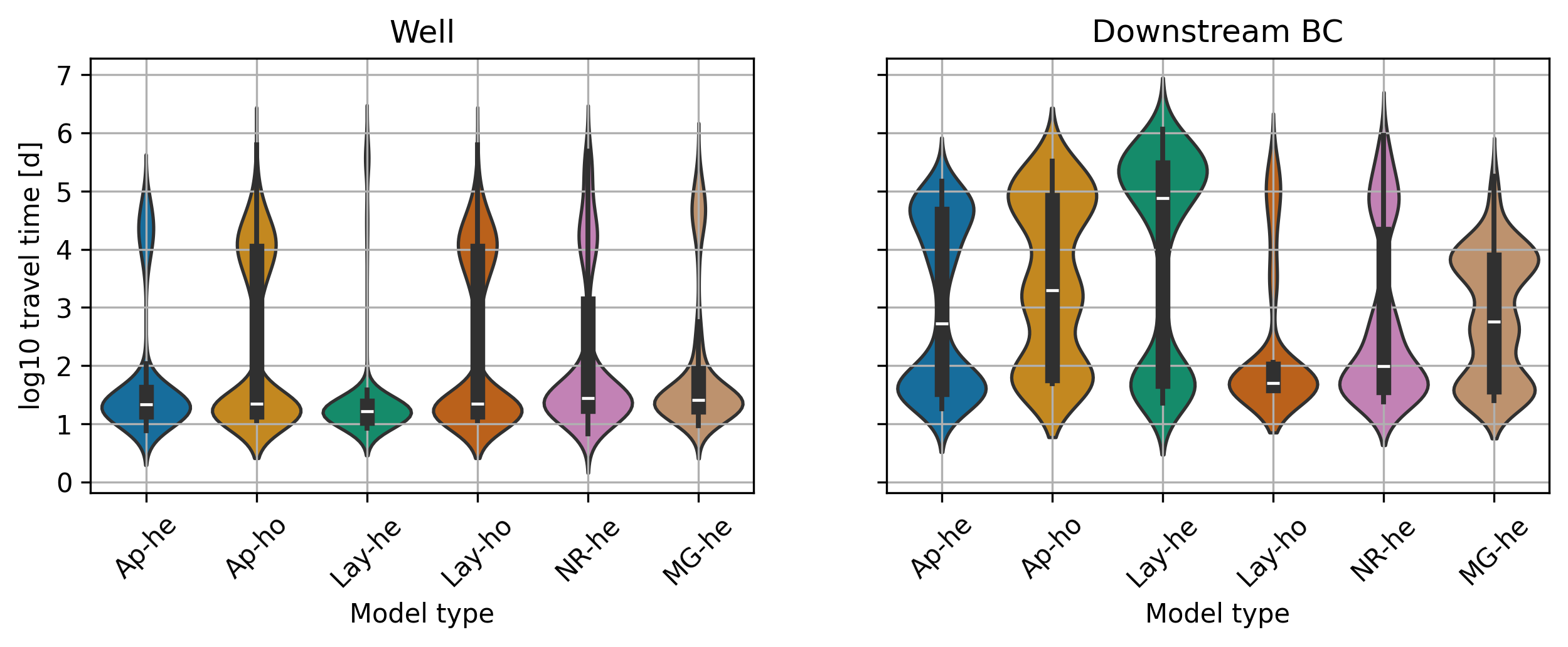
[ ]: